How to find outliers in measured data using the z-score, modified z-score (MAD), IQR fences, the Hampel filter, and the Grubbs and generalized ESD tests—and why one outlier can hide another.
Contents
What Is an Outlier? Which Points Do Not Belong?
Almost every measured record has a few values that look wrong: a temperature sensor that reads 24 °C for one second in a room at 20 °C, a weighing where a digit was entered incorrectly, or a network ping that takes ten times longer than the rest. Some are glitches to remove; others are the most interesting events in the record. Either way, they have to be found first, using a rule rather than by eye.
An outlier is a point far from the rest of the data. "Far" requires two things: a center that says where the data usually lies, and a spread that says how far a normal point typically strays from it. Each point gets a score—its distance from the center measured in units of spread—and a point whose score passes a threshold is flagged.
The catch is in the center itself (Fig 1). The usual center, the mean, is the average of every point, including the outlier, so the outlier pulls the center toward itself. The median, the middle value, does not move.
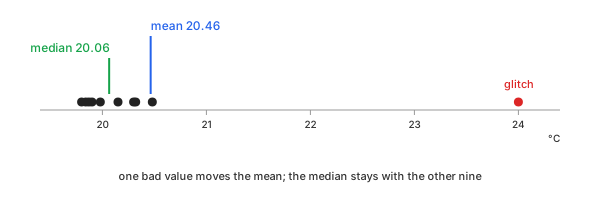
Fig 1. One bad value moves the mean; the median stays with the others
Take an example: three columns sampled once a second for 120 seconds—120 rows. The example has three purposes.
- $y_1$, glitches on a steady signal. A room thermometer at 20 °C with a little noise (standard deviation 0.2 °C) and three glitches: +4.0 °C at 30 s, −1.0 °C at 75 s, and +0.9 °C at 100 s.
- $y_2$, glitches on a drifting signal. The same room warming by 0.03 °C per second, with three glitches of ±1.0 °C at 20 s, 58 s, and 95 s.
- $y_3$, no glitch at all. A server's response time in milliseconds: always positive, usually near 10 ms, and occasionally two or three times that. Every value is genuine.
Table 1 shows ten seconds of $y_1$ around the large glitch, along with the two deviations from which every method below starts.
| t (s) | $y_1$ (°C) | $y_1 - \bar{y}$ | $(y_1 - \bar{y})^2$ | $|y_1 - \tilde{y}|$ |
|---|---|---|---|---|
| 25 | 19.98 | −0.484 | 0.2343 | 0.085 |
| 26 | 19.87 | −0.594 | 0.3528 | 0.195 |
| 27 | 20.32 | −0.144 | 0.0207 | 0.255 |
| 28 | 20.30 | −0.164 | 0.0269 | 0.235 |
| 29 | 20.48 | 0.016 | 0.0003 | 0.415 |
| 30 | 24.00 | 3.536 | 12.5033 | 3.935 |
| 31 | 19.84 | −0.624 | 0.3894 | 0.225 |
| 32 | 19.90 | −0.564 | 0.3181 | 0.165 |
| 33 | 19.80 | −0.664 | 0.4409 | 0.265 |
| 34 | 20.15 | −0.314 | 0.0986 | 0.085 |
| sum | 14.3852 | |||
Table 1. Ten seconds of $y_1$, t = 25 to 34 s: the glitch in bold
Here $\bar{y} = 20.464$ is the mean of the ten values and $\tilde{y} = 20.065$ is their median. Chart 1 shows all 120 rows of the three columns.
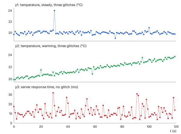
Chart 1. The example: two thermometers with glitches, and a skewed record without any
The task: flag the three glitches in $y_1$ and the three in $y_2$, and nothing in $y_3$—using only the data.
Methods
Six methods, in three pairs: two scores against the whole record (mean or median), two that need no normal distribution at all or look only nearby, and two formal tests.
Z-Score
In plain words. Distance from the mean, measured in standard deviations. Both are computed from every point, including the outliers: the baseline that the other five methods improve upon.
Control parameters. threshold ($t$, default 3):
the largest $|z|$ still counted as normal. For normally distributed data, 0.27% of points
exceed 3 by chance.
Basic idea. The standard score of point $y_i$, with the mean $\bar{y}$ and the sample standard deviation $s$ of all $N$ points (Math 1):
Math 1.
Point $i$ is flagged when $|z_i| > t$.
Example. The ten values in Table 1 add up to 204.64; the squared deviations add up to 14.3852 (Math 2):
Math 2.
The glitch at 30 s then scores (Math 3):
Math 3.
Not flagged—a value 4 °C off in a room whose other readings stay within 0.5 °C of 20 °C. The glitch made its own yardstick: its squared deviation, 12.5033, is 87% of the sum in Table 1, so $s$ is five times what the other nine give (0.2482). Over all 120 rows, the same glitch scores 9.106 and is flagged, but the two small glitches score −2.348 and 2.005 and are not (Chart 2, blue lines).
Important characteristics. Both the center and the spread are computed from every point, including the outliers.
Advantages
- Familiar and quick to compute.
- A clear meaning for normally distributed data: the chance of exceeding $t$ is known.
Disadvantages
- The outlier inflates $s$ and hides itself and others (see Masking).
- A record of 10 or fewer points can never reach 3 (see The Z-Score Ceiling).
Modified Z-Score (MAD)
In plain words. The z-score with the median in place of the mean and the median absolute deviation (MAD) in place of the standard deviation. The same score, but based on a center and spread that outliers cannot drag.
Control parameters. threshold ($t$, default 3.5, the
value recommended by Iglewicz and Hoaglin).
Basic idea. With $\tilde{y}$ as the median of all points and the median absolute deviation MAD as the median of the distances $|y_i - \tilde{y}|$ (Math 4):
Math 4.
The factor 0.6745 puts $M$ on the scale of $z$: for normally distributed data, MAD is 0.6745 standard deviations, so $\mathrm{MAD} / 0.6745$ estimates the same spread as $s$.
Example. In Table 1, the median of the ten values is $(19.98 + 20.15) / 2 = 20.065$. The distances $|y_i - \tilde{y}|$ in the last column, in order, are 0.085, 0.085, 0.165, 0.195, 0.225, 0.235, 0.255, 0.265, 0.415, 3.935; their median is 0.230 (Math 5):
Math 5.
Flagged, and by a wide margin. The glitch's own distance, 3.935, is the largest of the ten, and the median of the ten ignores how large it is. Over all 120 rows, all three glitches of $y_1$ are flagged: 16.433, −4.006, and 3.761. Chart 2 shows both rules on the whole of $y_1$: the band of the z-score, mean ± $3s$, is wide enough to let the two small glitches through; the band of the modified z-score, median ± $3.5\,\mathrm{MAD} / 0.6745$, is not.
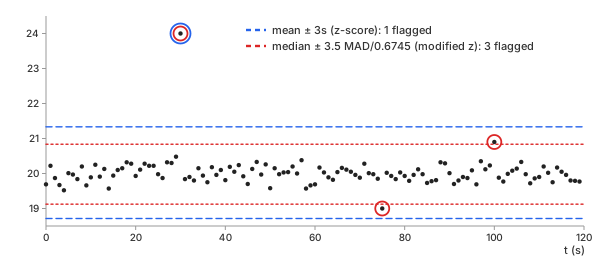
Chart 2. $y_1$: the z-score band flags 1 glitch, the modified z-score band flags all 3
Important characteristics. Half of the points can be outliers before the median or the MAD moves far (see Breakdown Point).
Advantages
- Not masked: one large outlier does not hide a small one.
- The same simple form as the z-score, with no table to look up.
Disadvantages
- MAD is 0 when more than half of the values are identical, and every other value then scores infinitely far.
- Still assumes a symmetric distribution around one center.
IQR: Tukey's Fences
In plain words. Only the middle 50% of the data sets the scale: no mean, no standard deviation, and no normal distribution assumed. Unlike the two z-scores, it is a fence around the bulk, not a score from one center. This is the rule behind the dots of a box plot.
Control parameters. threshold ($k$, default 1.5):
how many interquartile ranges the fences extend beyond the quartiles. Tukey used 3 for
"far out."
Basic idea. With $Q_1$ and $Q_3$ as the first and third quartiles (25% and 75% of the points lie below them) and the interquartile range $\mathrm{IQR} = Q_3 - Q_1$ (Math 6):
Math 6.
A point below the lower fence or above the upper one is flagged; a point exactly on
a fence is not. The quartiles are interpolated linearly between the sorted values, as
numpy.percentile does by default.
Example. The ten values in Table 1, sorted: 19.80, 19.84, 19.87, 19.90, … 20.32, 20.48, 24.00. The first quartile falls a quarter of the way from the third value to the fourth, and the third quartile three quarters of the way from the seventh to the eighth (Math 7):
Math 7.
24.00 lies above 20.971: flagged. Over all 120 rows, the fences of $y_1$ are 19.371 and 20.621, and exactly the three glitches lie outside (Chart 3, left).
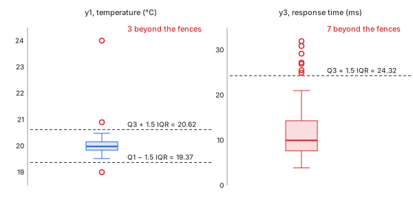
Chart 3. Tukey's fences on $y_1$ (3 beyond) and on $y_3$ (7 beyond)
On $y_3$, the same rule flags 7 of 120 response times, every one of them genuine (Chart 3, right; see Skewed Data).
Important characteristics. Quartiles, like the median, ignore how far the extreme points lie, and the fences need no assumption of a normal distribution.
Advantages
- Robust and familiar from every box plot.
- No standard deviation, so nothing for an outlier to inflate.
Disadvantages
- In a skewed distribution, the long side gets flagged wholesale.
- The fences are the same for the whole record, so drift defeats them as it defeats the z-score.
Hampel Filter
In plain words. A local modified z-score: each point is judged against the median and MAD of a short window of its neighbors in time, rather than those of the whole record. The center follows the signal, so drift no longer hides a spike.
Control parameters. window ($k$, default 5): the
number of points on each side, so the window holds $2k + 1$ points; it is cut short at
the two ends of the record. threshold ($t$, default 3): how many scaled
MADs a point may stray from its window's median.
Basic idea. For each point $i$, the median $m_i$ of its window and the window's MAD, scaled by $1.4826 = 1 / 0.6745$ into a standard deviation $S_i$ (Math 8):
Math 8.
The score is $(y_i - m_i) / S_i$. The line of window medians $m_i$ is a median filter; the Hampel filter adds a band around it. A window whose MAD is 0 has no spread to judge by, and its point is not flagged.
Example. $y_2$ rises by 3.6 °C over the record, so its standard deviation, 1.061 °C, measures the rise rather than the noise. The z-score band, mean ± $3s$, spans 18.6 to 25.0 °C and holds every point; the modified z-score and the IQR fences flag nothing either. With $k = 5$, the Hampel filter compares each point with the 11 around it (Chart 4):
| t | $y_2$ | window median $m_i$ | $S_i$ | score | global $z$ |
|---|---|---|---|---|---|
| 20 s | 21.53 | 20.620 | 0.2076 | 4.384 | −0.229 |
| 58 s | 20.84 | 21.730 | 0.1779 | −5.002 | −0.879 |
| 95 s | 23.57 | 22.840 | 0.2076 | 3.517 | 1.694 |
Table 2. The three glitches of $y_2$: Hampel scores against global z-scores
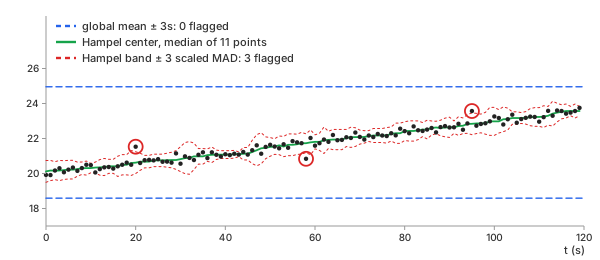
Chart 4. $y_2$: the Hampel band follows the drift and flags the 3 glitches; the global band flags none
Important characteristics. Each point has its own center and spread, so a slow trend and slow changes in noise do not matter. The window has to be longer than a glitch and shorter than the changes in the signal.
Advantages
- Finds spikes on drifting or wandering signals.
- Its window median is a natural replacement for a flagged point.
Disadvantages
- Only 11 points estimate each spread, so noise alone is flagged now and then.
- A burst of glitches longer than half the window becomes the window's median, and nothing is flagged.
Grubbs' Test
In plain words. A statistical test built on the normal distribution: could $N$ normal points produce the farthest one by chance? Unlike the four scores above, the line is not a fixed threshold but a chosen false-alarm rate, and it changes with $N$.
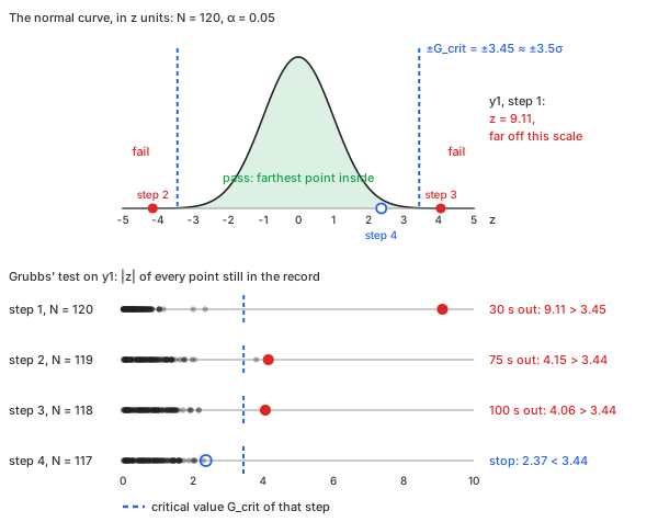
Fig 2. Grubbs' test: the record passes while its farthest point stays inside ±G_crit on the normal curve; a point beyond it is removed and the test repeats
Control parameters. alpha ($\alpha$, default 0.05):
the chance, per test, of flagging a point when the data contain no outlier at all.
Basic idea. Grubbs' test takes the largest $|z|$ in the record as its statistic $G$ and compares it with a critical value from the $t$-distribution with $N - 2$ degrees of freedom (Math 9):
Math 9.
- Why a pass condition: every record has a farthest point, even clean normal data. Removing it every time would strip normal points forever, so the test needs a line for how far the farthest point may lie and still be normal.
- Pass condition: the record passes, with no outlier, while its farthest point stays inside mean ± $G_{\text{crit}} \cdot s$ (Fig 2, top).
- $G_{\text{crit}}$: the farthest that chance alone
reaches; $N$ normal points with no outlier break out of the band only with probability
$\alpha$. It widens with $N$, for $\alpha = 0.05$:
- $N = 10$: ±2.290
- $N = 37$: ±3.003
- $N = 120$: ±3.445
- 3.5σ and $\alpha = 0.05$: at $N = 120$, $G_{\text{crit}} = 3.445$,
so the pass band is about ±3.5σ of the normal distribution.
- per point: one normal point lands beyond ±3.5σ with a probability of 0.047%
- per record: among 120 normal points, at least one lands beyond it in 5.4% of records, about $\alpha$
- meaning: $\alpha = 0.05$ is the chance that a clean record is wrongly flagged; for 120 points, ±3.5σ is the band where that chance reaches 5%
If $G > G_{\text{crit}}$, the point is an outlier; it is removed, and the test runs again on the remaining $N - 1$ points, with a new mean, a new $s$, and a new critical value.
Example. $y_1$, all 120 points, $\alpha = 0.05$ (Table 3):
| step | N | mean | $s$ | farthest point | $G$ | $G_{\text{crit}}$ |
|---|---|---|---|---|---|---|
| 1 | 120 | 20.0248 | 0.4365 | 30 s, 24.00 | 9.106 | 3.445 |
| 2 | 119 | 19.9914 | 0.2390 | 75 s, 19.00 | 4.148 | 3.442 |
| 3 | 118 | 19.9998 | 0.2217 | 100 s, 20.90 | 4.061 | 3.440 |
| 4 | 117 | 19.9921 | 0.2062 | 29 s, 20.48 | 2.366 | 3.437 |
Table 3. Grubbs' test on $y_1$, step by step: three outliers, then a stop
Each removal shrinks $s$—from 0.4365 to 0.2062—and lets the next glitch stand out. At step 4, the farthest point left, a normal reading, scores 2.366, below 3.437, and the test stops: three outliers, the three glitches.
Important characteristics. It is a real hypothesis test: with $\alpha = 0.05$, clean normal data pass without a single flag 95% of the time, whatever $N$ is. The threshold grows with $N$ by itself, unlike a fixed 3.
Advantages
- A false-alarm rate you choose, instead of a threshold you guess.
- Removing one point at a time undoes the masking of the z-score.
Disadvantages
- Assumes the data without outliers are normally distributed.
- Stops at the first test that fails: two outliers of the same size can mask each other, and the test finds neither.
Generalized ESD Test
In plain words. Grubbs' test extended to multiple outliers: up to $r$ suspects are removed first, and the count is decided afterwards. Where Grubbs' test stops at the first failure, it looks past it, so outliers that mask each other are still found.
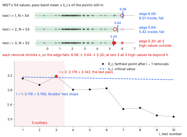
Fig 3. Generalized ESD: each removal shrinks the band; at the last pass all three high values lie outside it
Control parameters. maxOutliers ($r$, default 10): an
upper bound on the number of outliers; alpha ($\alpha$, default 0.05).
Basic idea. The generalized extreme studentized deviate (ESD) test of Rosner computes, for $i = 1, \dots, r$, the statistic $R_i$ of the farthest point after $i - 1$ removals and a critical value $\lambda_i$ (Math 10):
Math 10.
- Why count afterwards: Grubbs' pass condition can be fooled. Two or three outliers of similar size inflate $s$ together, so the farthest one alone looks normal and Grubbs' test stops before finding any (Fig 3, $i = 1$). Each removal shrinks $s$, so the band shrinks faster than the next value falls: on NIST's data, its edge drops from 6.06 to 5.64 to 5.30, and at test 3 all three high values lie beyond it.
- Pass condition per test: $R_i \le \lambda_i$, Grubbs' band applied to the $N - i + 1$ points left; $\lambda_1$ is Grubbs' $G_{\text{crit}}$.
- Count: the largest $i$ with $R_i > \lambda_i$, even if a
smaller $i$ fails. On NIST's 54 values (Fig 3):
- $i = 1$: 3.118 < 3.158, fails; Grubbs' test stops here
- $i = 2$: 2.942 < 3.151, fails
- $i = 3$: 3.179 > 3.143, the last pass: 3 outliers
- $\alpha = 0.05$: the chance that a clean record, with no outlier, reports any outlier across all $r$ tests is about 5%, as for Grubbs' test.
Example. $y_1$ with $r = 10$ and $\alpha = 0.05$ (Table 4):
| $i$ | removed point | $R_i$ | $\lambda_i$ |
|---|---|---|---|
| 1 | 30 s, 24.00 | 9.106 | 3.445 |
| 2 | 75 s, 19.00 | 4.148 | 3.442 |
| 3 | 100 s, 20.90 | 4.061 | 3.440 |
| 4 | 29 s, 20.48 | 2.366 | 3.437 |
| 5 | 4 s, 19.52 | 2.316 | 3.434 |
| … | … | … | … |
| 10 | 97 s, 20.35 | 1.887 | 3.419 |
Table 4. Generalized ESD on $y_1$: the largest $i$ with $R_i > \lambda_i$ is 3
On $y_1$, the answer equals Grubbs': three outliers. The difference shows on data where two outliers mask each other. NIST's example, 54 values from Rosner's paper, gives $R_1 = 3.118 < \lambda_1 = 3.158$, so Grubbs' test stops at once and finds nothing; the generalized ESD test goes on, finds $R_3 = 3.179 > \lambda_3 = 3.143$, and reports three outliers.
Important characteristics. Only an upper bound $r$ is needed, not the exact number of outliers, and the critical values account for the number of tests made.
Advantages
- Not fooled when outliers mask each other.
- The recommended test for several outliers in normal data (NIST).
Disadvantages
- Assumes the data without outliers are normally distributed.
- Needs a guess of $r$; NIST notes that the critical values are reliable from about 15 points up.
The Six Side by Side
The six methods differ in five choices (Table 5): which points form the center, what the center is, whether an outlier can move it, how the line between normal and outlier is drawn, and how many outliers one test can report.
| choice | one side | other side |
|---|---|---|
| global or local | global: z-score, modified z-score, IQR, Grubbs, ESD | local: Hampel |
| mean or median | mean: z-score, Grubbs, ESD | median: modified z-score, IQR (quartiles), Hampel (window median) |
| robust or not | not robust: z-score, Grubbs, ESD | robust: modified z-score, IQR, Hampel |
| threshold or test | threshold: z-score, modified z-score, IQR, Hampel | statistical test: Grubbs, ESD |
| single or multiple | single: Grubbs, one point per test, repeated | multiple: z-score, modified z-score, IQR, Hampel, ESD (up to $r$) |
Table 5. Five ways the six methods differ
Mean and median split the methods the same way robust and not robust do: the median ignores how far an outlier lies, the mean does not. The two tests make up for a center that moves by removing one point at a time, so a large outlier stops inflating $s$ once it is out.
Which One Should You Choose?
| your data | use | in the example |
|---|---|---|
| steady, roughly normal, one obvious outlier | z-score | $y_1$: 1 of 3 glitches |
| steady, several outliers of different sizes | modified z-score | $y_1$: 3 of 3 |
| no assumption of a normal distribution, a box plot to show | IQR fences | $y_1$: 3 of 3; $y_3$: 7 false alarms |
| drifting or wandering signal, spikes | Hampel filter | $y_2$: 3 of 3, global methods 0 |
| a formal answer for normal data, one or few outliers | Grubbs' test | $y_1$: 3 in 3 steps |
| a formal answer, several outliers that may mask each other | generalized ESD | $y_1$: 3; NIST data: 3 where Grubbs finds 0 |
Table 6. Which method for which data
The basic calculator computes the z-score, the modified z-score, the IQR fences, and the Hampel filter in your browser. The advanced calculator adds Grubbs' test and the generalized ESD test and any number of columns, computed on the server.
Key Ideas
Each method is a one-line formula. Using them well takes six ideas.
Masking: One Outlier Hides Another
In $y_1$ the large glitch raises the standard deviation of the whole record from 0.2390 (without it) to 0.4365. With the large glitch in, the small glitches score −2.348 and 2.005; with it removed, −4.148 and 3.801. One outlier masks the others by widening the yardstick all of them are measured with (Chart 2).
Two cures appear above: a center and spread that the outlier cannot move (median and MAD, quartiles), or removing outliers one at a time and measuring again (Grubbs, generalized ESD).
The Z-Score Ceiling: Small Records Never Reach 3
Put one point as far out as you like among $N - 1$ equal ones. It drags the mean and inflates $s$ with it, and its z-score can never exceed (Math 11):
Math 11.
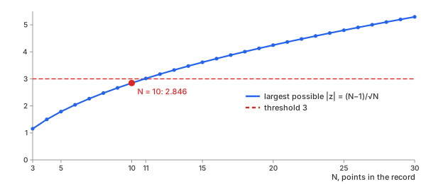
Chart 5. The largest $|z|$ a record of $N$ points can reach
For $N = 10$ the ceiling is 2.846, and for $N = 11$ it is 3.015. That is why the glitch of Table 1 scored 2.797: with ten points, a threshold of 3 cannot flag anything, however wrong. The other five methods have no such ceiling.
Breakdown Point: How Many Bad Points Before the Center Moves
The breakdown point of an estimate is the share of points that can be replaced by arbitrary values before the estimate can be moved arbitrarily far. For the mean it is 0%: one point is enough. For the median and the MAD it is 50%. Table 7 replaces more and more points of $y_1$ with 24.00 °C:
| bad points | mean | median | $s$ | MAD |
|---|---|---|---|---|
| 0 (0%) | 20.025 | 19.980 | 0.437 | 0.165 |
| 1 (0.8%) | 20.056 | 19.980 | 0.567 | 0.165 |
| 12 (10%) | 20.426 | 20.015 | 1.272 | 0.175 |
| 36 (30%) | 21.235 | 20.135 | 1.863 | 0.290 |
| 48 (40%) | 21.622 | 20.210 | 1.993 | 0.450 |
| 61 (50.8%) | 22.032 | 24.000 | 2.018 | 0.000 |
Table 7. $y_1$ with more and more points set to 24.00 °C
The mean moves with every bad point; the median stays within 0.23 °C up to 40% and only jumps once the bad points are the majority—at which point they are no longer the outliers.
Global or Local: Drift Hides Spikes
The z-score, the modified z-score, the IQR fences, and both tests share one center for the whole record. On $y_2$ that center is wrong almost everywhere: the room warms by 3.6 °C, and every glitch lies well inside the spread of the trend (Chart 4). Two fixes:
- Remove the trend first, then run any method on the residuals (Detrending & Baseline Correction).
- Judge locally, with the Hampel filter: its window median follows the signal like a median filter, and its band follows the local noise.
Skewed Data: A Long Tail Is Not a List of Outliers
Response times, particle sizes, incomes, and concentrations are positive and skewed: most values are small, and a long tail stretches to the right. $y_3$ is such a record, with no glitch in it, and yet the z-score flags 2 of its 120 values, the modified z-score 3, the IQR fences 7 (Chart 3, right), and the Hampel filter 12. Each rule assumes a symmetric distribution and reads the tail as a fault.
The cure is to work on a scale where the data are symmetric. For a log-normal record like $y_3$, take the logarithm first: the skewness drops from 1.352 to 0.208, and neither the z-score nor the IQR fences flag a single value of $\log y_3$.
Replace, Do Not Delete
Flagging a point is a statistical statement; removing it is a decision. Before either, ask what the point is—a glitch, a real event, or a sign that the method's assumptions do not hold, as in $y_3$.
For a time series, a deleted row also leaves a gap. Every method that counts samples—a Fourier transform, a digital filter, a cross-correlation—then treats two points a second apart as neighbors. Replace a flagged value instead: with the median of its window (Hampel) or of the record, or by linear interpolation between its two neighbors.
Score against a center the outlier cannot move—and decide afterwards.
REFs
NIST/SEMATECH e-Handbook, Detection of Outliers NIST/SEMATECH e-Handbook, Grubbs' Test for Outliers NIST/SEMATECH e-Handbook, Generalized ESD Test for Outliers SciPy scipy.stats.zscore SciPy scipy.stats.median_abs_deviation NumPy numpy.percentile Wikipedia, Outlier Wikipedia, Median absolute deviation Wikipedia, Interquartile range Wikipedia, Grubbs's test Wikipedia, Robust statistics Smoothing Methods: Moving Average, EWMA, Savitzky-Golay, Gaussian, Median Detrending & Baseline Correction: How to Remove Drift from Measured Data