How the Fourier transform turns samples over time into amplitudes over frequency - the discrete Fourier transform (DFT) that defines it, the fast Fourier transform (FFT) that computes it fast, and the four things that decide what a spectrum can show.
Contents
What is the Fourier transform: what frequencies are in my data
You have a column of numbers measured over time - a vibration sensor, a voltage, a sound level, a daily count. Plotted, it wiggles. The question this page answers is the one you actually have: which frequencies is that wiggle made of, and how strong is each one?
The idea behind the Fourier transform is that a signal can be rebuilt as a sum of sine waves, each with its own frequency and its own amplitude. The transform finds that recipe. It turns a list of values over time into a list of amplitudes over frequency - a spectrum. A tall bar in the spectrum means a strong frequency in your data; an empty stretch means there is nothing there (Fig 1).
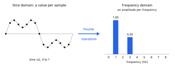
Fig 1. From time to frequency: the same data before and after the transform
Take an example. Sample two waves 16 times a second for one second - 16 points each - and add them: a 1 Hz wave of amplitude 1.0 and a 3 Hz wave of amplitude 0.5. The sum is what a sensor would record (Table 1).
| n | t (s) | 1 Hz | 3 Hz | sum |
|---|---|---|---|---|
| 0 | 0.0000 | 0.000 | 0.000 | 0.000 |
| 1 | 0.0625 | 0.383 | 0.462 | 0.845 |
| 2 | 0.1250 | 0.707 | 0.354 | 1.061 |
| 3 | 0.1875 | 0.924 | -0.191 | 0.733 |
| 4 | 0.2500 | 1.000 | -0.500 | 0.500 |
| 5 | 0.3125 | 0.924 | -0.191 | 0.733 |
| 6 | 0.3750 | 0.707 | 0.354 | 1.061 |
| 7 | 0.4375 | 0.383 | 0.462 | 0.845 |
| 8 | 0.5000 | 0.000 | 0.000 | 0.000 |
| 9 | 0.5625 | -0.383 | -0.462 | -0.845 |
| 10 | 0.6250 | -0.707 | -0.354 | -1.061 |
| 11 | 0.6875 | -0.924 | 0.191 | -0.733 |
| 12 | 0.7500 | -1.000 | 0.500 | -0.500 |
| 13 | 0.8125 | -0.924 | 0.191 | -0.733 |
| 14 | 0.8750 | -0.707 | -0.354 | -1.061 |
| 15 | 0.9375 | -0.383 | -0.462 | -0.845 |
Table 1. The example: 16 samples of a 1 Hz wave, a 3 Hz wave and their sum
The bold rows show the amplitudes. At $n = 4$ and $n = 12$ each wave sits at its full height - $\pm 1.0$ for the 1 Hz wave, $\pm 0.5$ for the 3 Hz wave. At $n = 8$ both cross zero, halfway through the second.
Chart 1 plots all three data sets at every sample point. Only the black sum is what you get to measure; the two colored waves are hidden inside it. The same example is used for the rest of this page, so every number can be checked against it.
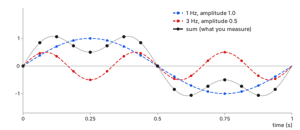
Chart 1. The three data sets of Table 1 at every sample point
And Chart 2 is its spectrum. Two bars, exactly where the two tones are, exactly as tall as their amplitudes: 1.0 at 1 Hz and 0.5 at 3 Hz. Nothing anywhere else.
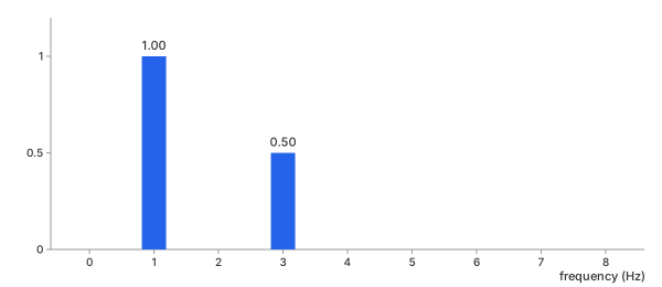
Chart 2. The spectrum of the sum: amplitude per frequency
Getting from Chart 1 to Chart 2 is the whole job. The rest of this page is how that is done, how to do it fast, and the four things that decide what a spectrum can and cannot show you. The way back, from Chart 2 to Chart 1, is the inverse Fourier transform.
Methods
There are two ways to compute the same spectrum. The DFT is the definition itself, computed term by term. The FFT is an algorithm that produces the identical numbers with far less work. They are not two different answers; they are two routes to one answer. On this data they agree to within $2 \times 10^{-14}$, which is floating-point round-off and nothing else.
DFT (direct sum)
In plain words. For every frequency you want to check, hold a test wave of that frequency up against your data, multiply them sample by sample, and add the products up. If your data contains that frequency, the products mostly agree in sign and the sum is large. If it does not, they cancel and the sum is zero.
Basic idea. With $N$ samples $y_0, \dots, y_{N-1}$, the discrete Fourier transform gives one complex number $Y_k$ for each frequency bin $k$ (Math 1). The second line writes the test wave with the twiddle factor $W_N$, the form the FFT below is built on:
Math 1.
The factor $W_N^{kn}$ is the test wave: a cosine and a sine of frequency $k$, packed into one complex number. Bin $k$ sits at frequency $k \cdot f_s / N$, where $f_s$ is the sampling rate - with 16 samples at 16 per second, bin $k$ is exactly $k$ Hz.
Here is the whole procedure by hand, on the same 16 samples as the example above ($N = 16$) - the data is in Table 1, plotted in Chart 1 - for bins 1, 2 and 3, that is, 1 Hz, 2 Hz and 3 Hz.
Step 1 - split the test wave. Since $e^{-i\theta} = \cos\theta - i\sin\theta$, each bin is two ordinary sums, one against a cosine and one against a sine (Math 2):
Math 2.
Step 2 - multiply every sample by both test waves. Each sample $y_n$ (the sum column of Table 1) times $\cos(2\pi k n/16)$ and times $\sin(2\pi k n/16)$, in Table 2:
| n | $y_n$ | cos (k=1) | sin (k=1) | cos (k=2) | sin (k=2) | cos (k=3) | sin (k=3) |
|---|---|---|---|---|---|---|---|
| 0 | 0.000 | 0.000 | 0.000 | 0.000 | 0.000 | 0.000 | 0.000 |
| 1 | 0.845 | 0.780 | 0.323 | 0.597 | 0.597 | 0.323 | 0.780 |
| 2 | 1.061 | 0.750 | 0.750 | 0.000 | 1.061 | -0.750 | 0.750 |
| 3 | 0.733 | 0.280 | 0.677 | -0.518 | 0.518 | -0.677 | -0.280 |
| 4 | 0.500 | 0.000 | 0.500 | -0.500 | 0.000 | 0.000 | -0.500 |
| 5 | 0.733 | -0.280 | 0.677 | -0.518 | -0.518 | 0.677 | -0.280 |
| 6 | 1.061 | -0.750 | 0.750 | 0.000 | -1.061 | 0.750 | 0.750 |
| 7 | 0.845 | -0.780 | 0.323 | 0.597 | -0.597 | -0.323 | 0.780 |
| 8 | 0.000 | 0.000 | 0.000 | 0.000 | 0.000 | 0.000 | 0.000 |
| 9 | -0.845 | 0.780 | 0.323 | -0.597 | -0.597 | 0.323 | 0.780 |
| 10 | -1.061 | 0.750 | 0.750 | 0.000 | -1.061 | -0.750 | 0.750 |
| 11 | -0.733 | 0.280 | 0.677 | 0.518 | -0.518 | -0.677 | -0.280 |
| 12 | -0.500 | 0.000 | 0.500 | 0.500 | 0.000 | 0.000 | -0.500 |
| 13 | -0.733 | -0.280 | 0.677 | 0.518 | 0.518 | 0.677 | -0.280 |
| 14 | -1.061 | -0.750 | 0.750 | 0.000 | 1.061 | 0.750 | 0.750 |
| 15 | -0.845 | -0.780 | 0.323 | -0.597 | 0.597 | -0.323 | 0.780 |
| sum | 0.000 | 8.000 | 0.000 | 0.000 | 0.000 | 4.000 |
Table 2. Each sample times the cosine and sine test waves, bins 1 to 3
Step 3 - add each column. The sin (k=1) column never goes negative: the data moves with the 1 Hz sine, so every product agrees and they pile up to 8. In the two k=2 columns every value is matched by its opposite, so they cancel to 0 - there is no 2 Hz in the data. The sin (k=3) column adds to 4. The cosine columns all cancel, because the data is built from sines only. Putting each pair of sums back into Math 2 gives Math 3:
Math 3.
Step 4 - turn each bin into an amplitude. Take the size $|Y_k|$, divide by $N$ and double (the reason for the doubling is in Reading the output below), in Math 4:
Math 4.
Those are the bars of Chart 2: 1.0 at 1 Hz, nothing at 2 Hz, 0.5 at 3 Hz. The other bins work the same way and all come out 0.
Important characteristics. Each of the $N$ bins needs a sum over all $N$ samples, so the DFT costs $N \times N = N^2$ complex multiplications. That is nothing at 16 samples and a real problem at a million.
Advantages
- It is the definition - nothing hidden, every number traceable to one sum
- Works for any $N$, with no reordering of the data
- You can compute only the bins you need, one at a time
Disadvantages
- $N^2$ cost: 1,024 samples already need about a million multiplications
- Repeats the same products over and over across different bins
FFT (Cooley-Tukey radix-2)
In plain words.
- Split one large DFT into two smaller DFTs
- Calculate the smaller ones
- Combine their results cheaply
- Repeat until each piece is a single sample
This is the idea behind almost every FFT in use, published by Cooley and Tukey in 1965.
Basic idea. For radix-2, split the samples into the even-numbered ones and the odd-numbered ones (Fig 2):
N-point DFT
    ↓
even samples + odd samples
    ↓
two (N/2)-point DFTs:  E_k and O_k
    ↓
combine with twiddle factors
    ↓
N-point result
Fig 2. Radix-2 FFT: one level of the split
Each half is a DFT of its own, $N/2$ points long - Math 1 applied to the even samples gives $E_k$, applied to the odd samples gives $O_k$ (Math 5):
Math 5.
The combining step is the butterfly (Math 6):
Math 6.
One multiplication, $W_N^k O_k$, serves two outputs: $Y_k$ takes it with a plus, $Y_{k+N/2}$ with a minus. So only $k = 0, \dots, N/2-1$ need a multiplication; the other half of the outputs costs a subtraction, almost nothing.
Example of Fig 2, with 32 samples. Count the complex multiplications, one split at a time (Math 7 to Math 9, each with its count below). The sample values do not matter here, only how many products each step needs.
Step 0 - the DFT itself
Math 7.
- 32 bins × 32 samples: $32^2 = 1{,}024$ multiplications
- twiddle values: only 32 different $W_{32}^{kn}$, repeating every 32
- total: 1,024
Step 1 - split once
Math 8.
- two 16-point DFTs, direct: $2 \times 16^2 = 512$
- $W_{32}^k O_k$ for $k = 0, \dots, 15$: 16
- $Y_{k+16}$: same products, a subtraction only: 0
- total: 528, about half of step 0
Step 2 - split again
Math 9.
- four 8-point DFTs, direct: $4 \times 8^2 = 256$
- $E_k$ and $O_k$ combines, 8 each: 16
- $Y_k$ combine, as in step 1: 16
- total: 288
Keep splitting until every DFT is a single sample, which costs nothing. That takes $\log_2 32 = 5$ splits and leaves only 5 combine levels of 16 multiplications: 80 in all, which is $\tfrac{N}{2}\log_2 N$ (Table 3).
| step | DFTs | size | direct DFTs | combines | total |
|---|---|---|---|---|---|
| 0 | 1 | 32 | 1,024 | 0 | 1,024 |
| 1 | 2 | 16 | 512 | 16 | 528 |
| 2 | 4 | 8 | 256 | 32 | 288 |
| 3 | 8 | 4 | 128 | 48 | 176 |
| 4 | 16 | 2 | 64 | 64 | 128 |
| 5 | 32 | 1 | 0 | 80 | 80 |
Table 3. FFT cost for 32 samples, split by split, in complex multiplications
Important characteristics. There are $\log_2 N$ combine levels of $N/2$ multiplications each, so the cost is $\tfrac{N}{2}\log_2 N$ complex multiplications instead of $N^2$. The result is the same DFT, not an approximation of it.
Advantages
- Much faster than the direct DFT, and the gap grows with $N$
- Exactly the same result as the DFT
- Scales to very large records
- Mature, heavily optimized libraries exist for it
Disadvantages
- More complicated than the direct sum
- Needs the data reordered into bit-reversed order before the first combine
- Radix-2 wants $N$ to be a power of 2; library FFTs handle any $N$ with other factorizations, so no padding is needed
- For very small $N$ the bookkeeping can cost more than it saves
Which one should you pick
For real data, the FFT - always. It gives the same numbers, and the saving is not a percentage but orders of magnitude (Chart 3, Table 4):
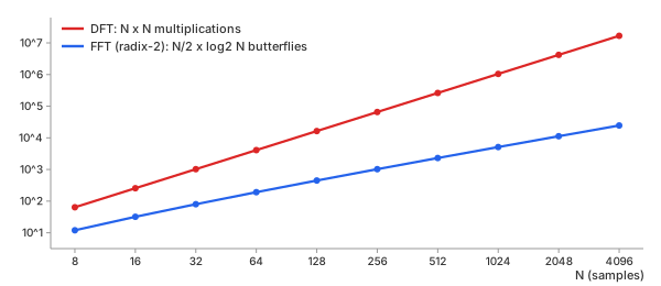
Chart 3. Cost against N: DFT vs FFT
| N | DFT: $N^2$ | FFT: $\tfrac{N}{2}\log_2 N$ |
|---|---|---|
| 16 | 256 | 32 |
| 1,024 | 1,048,576 | 5,120 |
| 65,536 | 4,294,967,296 | 524,288 |
Table 4. Cost in complex multiplications
The DFT still earns its place in two cases: when you are learning what the transform does, because every number traces back to one visible sum, and when you need only a handful of bins from a short record. That is why the basic calculator runs a DFT in your browser on up to 1,024 samples, and the advanced calculator offers the FFT for longer records.
Key ideas
The transform itself is exact. What limits a spectrum is how the data was recorded - and the first limit is why aliasing happens at all.
Why aliasing happens. Think of a film of a spinning wheel. The camera takes a picture 24 times a second. If the wheel turns almost a full circle between two pictures, the film shows it turning a little backwards - a slow wheel that is not there. Sampling does the same to a wave: it sees only where the wave is at each sample, never how many times it went round in between. A fast wave and a slow one that happen to sit at the same places at every sample look identical.
In the spectrum, this shows up as copies. The spectrum of sampled data is the true spectrum repeated at every multiple of the sampling rate $f_s$ (Fig 3). If the signal stays below $f_s / 2$, the copies stand apart and the real one can be read off. If it reaches past $f_s / 2$, the copies overlap - and that overlap is aliasing.
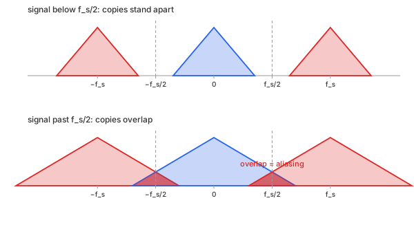
Fig 3. The sampled spectrum: copies at every multiple of $f_s$
Four parameters decide what a spectrum can show.
Sampling rate sets the top frequency (Nyquist, aliasing)
Sampling interval $T_s$ - the time between two samples. Sampling rate $f_s = 1 / T_s$ - how many samples per second. The two say the same thing: a short interval is a high rate.
- example: our data, $T_s = 0.0625$ s, so $f_s = 16$ samples per second (Table 1, Chart 1)
- good rate: above twice the fastest frequency in the signal. A 3 Hz wave at 16 per second - the dots follow the wave (Chart 4)
- bad rate: below twice the fastest frequency. The same 3 Hz wave at 4 per second - the dots trace a 1 Hz wave that is not there (Chart 5)
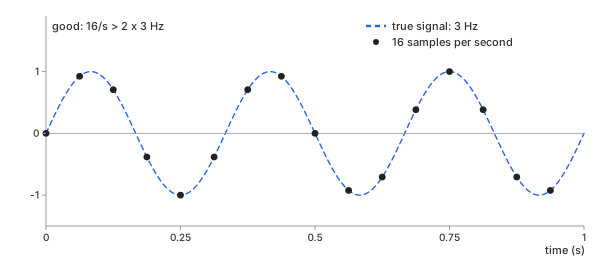
Chart 4. Good sampling rate: 3 Hz at 16 samples per second
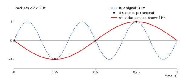
Chart 5. Bad sampling rate: 3 Hz at 4 samples per second, seen as 1 Hz
Nyquist frequency (folding frequency) $f_s / 2$ - the highest frequency a spectrum can show. Anything above it folds back to a lower one (Math 10):
Math 10.
- Chart 4: $f_s = 16$, Nyquist frequency 8 Hz. the 3 Hz wave is below it - shown as 3 Hz
- Chart 5: $f_s = 4$, Nyquist frequency 2 Hz. the 3 Hz wave is above it - folds to $|3 - 4| = 1$ Hz
The samples in Chart 5 really are the same as a 1 Hz wave's. At $t = n / 4$ (Math 11):
Math 11.
Filter before sampling, not after. Once a tone has folded, its samples are the same numbers as the alias's, so no digital filter can tell them apart - only an analog low-pass filter in front of the converter can. See Digital Filters: a filter cannot undo aliasing.
- once sampled at 4 per second: 1 Hz and 3 Hz cannot be told apart, by any method
- fix: before recording - sample above twice the fastest frequency, or filter it out first
Record length sets the spacing (frequency resolution)
Frequency resolution $\Delta f$ - the spacing between two bins, one over the length of the record (Math 12):
Math 12.
- example: two tones 0.5 Hz apart, 3 Hz and 3.5 Hz, amplitude 1.0 each, at 16 per second
- bad: 1 s record, 16 samples, $\Delta f = 16/16 = 1$ Hz - wider than the gap. one lumpy peak, 1.19 at 3 Hz, 0.63 at 4 Hz (Chart 6)
- good: 4 s record, 64 samples, $\Delta f = 16/64 = 0.25$ Hz - finer than the gap. two clean bars, 1.00 at 3 Hz and 1.00 at 3.5 Hz (Chart 7)
- fix: record longer. sampling faster raises the top frequency, not the spacing - Charts 4 and 5 are both 1 s records, both $\Delta f = 1$ Hz
A period needs no bins. When the record cannot be made longer and only the period of one repeating signal is wanted, autocorrelation reads it in seconds, between the bins - see Cross-Correlation: a period in a short record.
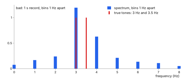
Chart 6. Bad resolution: 1 s record, bins 1 Hz apart
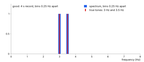
Chart 7. Good resolution: 4 s record, bins 0.25 Hz apart
Spectral leakage, and the window that tames it
Spectral leakage - a tone that does not complete a whole number of cycles in the record leaves a jump where the DFT joins the record's end to its start, and that jump spreads the tone into bins where there is no signal (spectral leakage).
- the DFT sees the record as if it repeats forever: end joined to start
- a 3.5 Hz tone over 1 s: 3.5 cycles, ends half-way round - the join jumps from −1 to +1 (Chart 8, top)
- that jump is not in the signal. the spectrum has to spend energy at many frequencies to build it
- with a window: both ends fade to 0, the join is smooth, the jump is gone (Chart 8, bottom)
Detrend first. A slow drift makes the same kind of jump: the record ends higher or lower than it starts. A window softens that jump, but the drift itself stays in the lowest bins. Remove it before the transform - see Detrending: trend and the FFT.
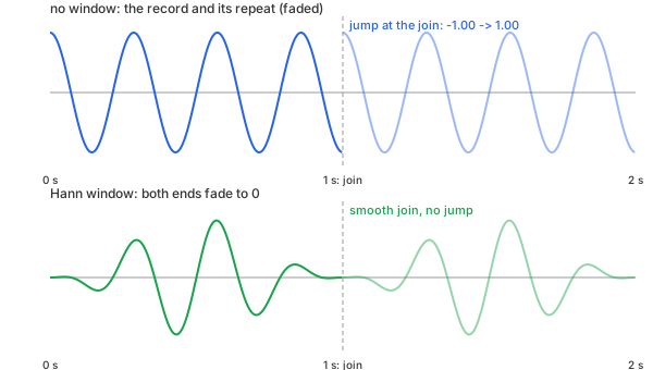
Chart 8. Why leakage happens: the record and its repeat, joined at 1 s
Window - a curve that fades to zero at both ends, multiplied into the data before the transform, so the end and the start meet at zero.
- example: a 3.5 Hz tone, halfway between two bins (Chart 9)
- no window (rectangular): the tone spills across every bin
- Hann window: the tone stays mostly in the two nearest bins, 3 and 4 Hz
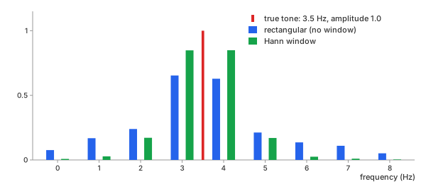
Chart 9. Leakage: a 3.5 Hz tone, no window vs Hann
The four windows differ in how they fade the record's ends (Chart 10):
- rectangular: no fade, the record as it is
- Hann: fades smoothly all the way to 0
- Hamming: fades almost to 0, stops at 0.08
- Blackman: the narrowest hump, 0 at both ends
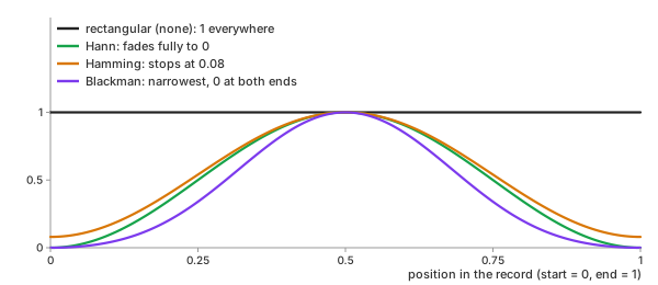
Chart 10. The four windows: the curve each one multiplies into the record
The more a window fades the ends, the less leakage - and the wider each peak. Every window trades one against the other (Table 5):
| window | peak width | leakage | use it when |
|---|---|---|---|
| rectangular (none) | narrowest | most | tones land exactly on bins, or the record is a transient that starts and ends at zero |
| Hann | medium | low | the default for unknown data |
| Hamming | medium | low near the peak | a strong tone sits next to a weaker one |
| Blackman | widest | lowest | a very weak tone must be seen beside a strong one |
Table 5. The four windows compared
When a window is needed
- tones not on a bin - almost every real record
- a continuous signal cut into a record: vibration, audio, a sensor stream
- a weak tone next to a strong one: leakage from the strong one hides it
When a window is not needed (rectangular)
- every tone completes a whole number of cycles in the record - on a bin, as in Table 1
- a transient that starts and ends at zero inside the record: a knock, a pulse, a decaying ring
- two equal tones very close together: every window widens the peaks, rectangular keeps them narrowest
A window also shrinks the data, so it shrinks the amplitudes. The calculators on this site correct for that: a sine of amplitude $A$ still reads $A$ whatever window you pick, as long as it lands on a bin.
Reading the output: magnitude, phase, the mirrored half
Each $Y_k$ is a complex number, and it carries two facts about frequency $k$:
- Magnitude $|Y_k|$ - how much of that frequency there is. Scaled as in Math 4, it reads directly as an amplitude.
- Phase $\arg Y_k$ - where in its cycle that wave starts. Our 1 Hz tone is a sine, and $Y_1 = -8i$ has a phase of $-90°$: a cosine shifted by a quarter turn, which is exactly what a sine is.
For real-valued data, the upper half of the bins is a mirror image of the lower half: $Y_{N-k}$ is the complex conjugate of $Y_k$, with the same magnitude. Chart 11 shows all 16 bins of our data:
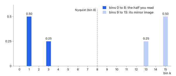
Chart 11. All 16 bins of the example: the mirrored half
Each tone appears twice - at bin $k$ and at bin $N-k$ - with half its amplitude in each: 0.5 and 0.5 for the 1 Hz tone, 0.25 and 0.25 for the 3 Hz one. The mirror holds no new information, so a spectrum is usually shown from bin 0 to bin $N/2$ only, with each bin doubled to put the two halves back together. That is the doubling in Math 4. Bin 0 (the mean of the data) and bin $N/2$ (the Nyquist bin) have no partner, so they are not doubled.
REFs
Inverse Fourier Transform (IDFT, IFFT): What Signal Does This Spectrum Make? - the inverse half of this page Cooley & Tukey (1965), "An Algorithm for the Machine Calculation of Complex Fourier Series" Harris (1978), "On the Use of Windows for Harmonic Analysis with the Discrete Fourier Transform" NumPy numpy.fft SciPy scipy.fft SciPy scipy.signal.get_window