How low-pass, high-pass, band-pass, and band-stop filters retain certain frequencies and reject others — Butterworth, Chebyshev, elliptic, Bessel, and FIR designs; cutoff frequency and filter order; and why zero-phase filtering eliminates phase lag.
Contents
What Is a Digital Filter? Which Frequencies Stay in My Signal?
A measured signal is usually a mixture of different components. An electrocardiogram (ECG) may contain 50 Hz or 60 Hz power-line hum, an accelerometer may pick up motor vibrations on top of the slow motion you want to measure, and every sensor adds broadband noise. When the wanted and unwanted components occupy different frequency ranges, they can be separated.
A digital filter does exactly that with sampled data: it preserves the frequencies you want and attenuates the rest (Fig 1).
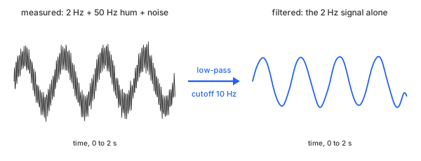
Fig 1. A low-pass filter keeps the slow wave and removes the hum and the noise
Every filter on this page computes each output sample $y[n]$ from the current and past input samples $x[n], x[n-1], \dots$ and, for most designs, from past output samples as well. The coefficients $b_k$ and $a_k$ are chosen by the filter design method (Math 1).
Math 1.
Math 1 represents one second-order section (SOS). A higher-order filter can be implemented as a chain of such sections, with each section feeding the next. For example, an order-4 filter consists of two second-order sections.
A filter is described by its frequency response: when a sine wave at frequency $f$ is applied as input, the output is a sine wave at the same frequency, scaled by the gain $G(f)$. A gain of 1 leaves that frequency unchanged, while a gain near 0 suppresses it. Gain is often expressed in decibels (dB) as $20 \log_{10} G$. Thus, $-20$ dB corresponds to one-tenth of the original amplitude, while $-60$ dB corresponds to one-thousandth.
A digital filter is not the same as smoothing. Smoothing is typically controlled by a window size measured in data points and often assessed visually; it primarily suppresses rapid variations. A filter, by contrast, is specified by a cutoff frequency in hertz. It can preserve slow variations, fast variations, or a band of frequencies in between. Its frequency response characterizes how each frequency is affected.
A filter is not the same as detrending, either. A high-pass filter attenuates frequencies below its cutoff, whereas detrending subtracts an estimated baseline from the signal.
Consider an example: a slow 2 Hz sine wave with an amplitude of 1, a 50 Hz hum with an amplitude of 0.5, and a small amount of random noise. The signal is sampled at 250 samples per second for 2 seconds, producing 500 data points (Table 1).
| t (s) | y (measured) | 2 Hz signal | 50 Hz hum |
|---|---|---|---|
| 0.000 | 0.0001 | 0.0000 | 0.0000 |
| 0.004 | 0.5556 | 0.0502 | 0.4755 |
| 0.008 | 0.3668 | 0.1004 | 0.2939 |
| 0.012 | −0.2327 | 0.1502 | −0.2939 |
| 0.016 | −0.3213 | 0.1997 | −0.4755 |
| 0.124 | 1.4277 | 0.9999 | 0.4755 |
| 0.248 | 0.3317 | 0.0251 | 0.2939 |
| 0.500 | 0.0363 | 0.0000 | 0.0000 |
| 1.000 | −0.3251 | 0.0000 | 0.0000 |
| 1.996 | −0.6336 | −0.0502 | −0.4755 |
Table 1. The example: 10 of its 500 points, with the two tones that make each one
The hum repeats every 5 samples, so it swings from 0 to ±0.48 within a few rows. The bold row is near the top of the slow wave, where the hum adds 0.48 on top of it. Chart 1 plots all 500 points.
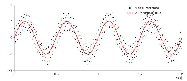
Chart 1. The example: measured data and the 2 Hz signal inside it
The task: recover the dashed 2 Hz wave from the data points.
Filter Types: Low-Pass, High-Pass, Band-Pass, and Band-Stop
The filter type determines which frequencies a filter preserves and which it attenuates (Fig 2):
- Low-pass preserves frequencies below the cutoff: the slow wave in the example.
- High-pass preserves frequencies above the cutoff: the hum and noise, while suppressing the slow wave.
- Band-pass preserves frequencies within a band defined by lower and upper cutoff frequencies: in this example, it can isolate the hum.
- Band-stop, also called a notch filter, attenuates frequencies within a specific band: in this example, it suppresses the hum while preserving the slow wave and most of the noise outside that band.
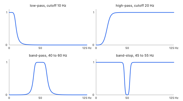
Fig 2. The four types, each a Butterworth filter of order 4
The frequency range extends up to 125 Hz, half the sampling rate. This limit, called the Nyquist frequency, is the highest frequency that can be uniquely represented by sampled data (see Nyquist).
Methods
Six filter designs, each representing a different trade-off between passband flatness, transition steepness, and time-domain behavior. For a fair comparison, all six methods are applied to the example using a low-pass filter with a cutoff frequency of 10 Hz and an order of 4. The FIR filter uses 101 taps.
Butterworth
In plain words. The flattest possible passband: the gain stays at 1 as long as possible, then falls smoothly through the cutoff, with no ripple anywhere.
Control parameters. order ($n$, below) determines how
steeply the gain falls; cutoff ($f_c$) is the frequency at which the gain has
dropped to $1/\sqrt{2}$, or −3 dB.
Basic idea. The digital Butterworth filter has a closed-form gain expression that depends on the sampling rate $f_s$ (Math 2).
Math 2.
Example. How much of the 50 Hz hum survives a cutoff of 10 Hz at order 4, with $f_s = 250$ Hz? First, calculate the ratio inside the brackets (Math 3).
Math 3.
Then raise it to the power $2n = 8$ (Math 4).
Math 4.
The hum's amplitude of 0.5 is reduced to 0.00046. At 2 Hz, the same formula gives a gain of 0.999999, so the slow wave passes essentially untouched.
Important characteristics. Monotonic: the gain only decreases as frequency increases, both within the passband and beyond the cutoff. It is the default choice when nothing else is known.
Advantages
- No ripple: frequencies well inside the passband retain their amplitude.
- Only one parameter besides the cutoff, with a formula that can be checked by hand.
Disadvantages
- A wider transition band than Chebyshev and elliptic designs of the same order.
- The step response overshoots by about 11% at order 4.
Chebyshev Type I
In plain words. Allow the passband gain to ripple slightly, and in return, the gain falls faster beyond the cutoff.
Control parameters. order ($n$); ripple
($r_p$, in dB), the maximum ripple allowed in the passband; and cutoff
($f_c$), the frequency at which the gain reaches the lower edge of the ripple band for the
last time.
Basic idea. The Chebyshev filter replaces Butterworth's power term with a Chebyshev polynomial $T_n$, which oscillates between −1 and 1 in the passband. Here, $\Omega = \tan(\pi f / f_s)$ is the prewarped frequency used in Math 2 (Math 5).
Math 5.
Example. With $r_p = 1$ dB (Math 6):
Math 6.
Every passband frequency has a gain between 0.8913 and 1. For even-order filters, the gain at 0 Hz is at the bottom of this range, so a constant signal is reduced to 89.13% of its original level.
Important characteristics. Steeper than Butterworth at the same order: −72.7 dB at 50 Hz versus −60.8 dB.
Advantages
- A sharper transition without increasing the order.
Disadvantages
- Passband ripple: amplitudes within the passband can vary by up to $r_p$, 1 dB here.
- More ringing: the step response overshoots by 22%.
Chebyshev Type II
In plain words. Keep the passband flat and put the ripple in the stopband instead, where the gain is already small.
Control parameters. order ($n$);
attenuation ($r_s$, in dB), the minimum attenuation anywhere in the stopband;
and cutoff ($f_c$), which here marks the start of the stopband
rather than the end of the passband.
Basic idea. The inverse Chebyshev filter effectively inverts the Chebyshev polynomial (Math 7).
Math 7.
Example. With $r_s = 40$ dB, the maximum gain in the stopband is $10^{-40/20} = 0.0100$, and $\varepsilon = 0.0100$. Because 10 Hz is already in the stopband, the passband ends at a lower frequency: the gain falls to −3 dB at 4.99 Hz (Chart 2).
Important characteristics. A flat passband, like Butterworth, combined with a steep transition, like Chebyshev Type I; the trade-off is a finite stopband floor.
Advantages
- No passband ripple and a fast transition into the stopband.
- The stopband floor is specified directly rather than discovered afterward.
Disadvantages
- The stopband attenuation never exceeds $r_s$: −42.3 dB at 50 Hz, compared with −60.8 dB for Butterworth.
- The cutoff parameter has a different meaning from that of the other methods on this page.
Elliptic
In plain words. Allow ripple in both bands in return for the steepest transition of any filter of a given order.
Control parameters. order ($n$); ripple
($r_p$); attenuation ($r_s$); and cutoff ($f_c$), the passband
edge, as in Chebyshev Type I.
Basic idea. The elliptic (Cauer) filter uses an elliptic rational function $R_n$, which oscillates in both the passband and the stopband (Math 8).
Math 8.
Example. With $r_p = 1$ dB and $r_s = 40$ dB, the gain stays between 0.8913 and 1 up to 10 Hz, then reaches −40 dB at about 15 Hz—the narrowest transition in Chart 2.
Important characteristics. Optimal in one sense only: it provides the narrowest transition for a given order and ripple specification. The trade-off is ripple in both bands and a less clean step response.
Advantages
- The lowest order for a given transition width: useful when computing power is limited.
Disadvantages
- Ripple in the passband and a finite stopband floor (−44.5 dB at 50 Hz).
- The most ringing on this page: a 24% overshoot.
Bessel
In plain words. Give up a sharp edge to preserve the shape of the signal: every frequency in the passband is delayed by nearly the same amount, so a pulse comes out looking like a pulse.
Control parameters. order ($n$); cutoff
($f_c$), set here as the −3 dB point, the same as for Butterworth.
Basic idea. The Bessel filter is built from a reverse Bessel polynomial $\theta_n$, chosen to make the group delay as flat as possible across the passband (Math 9).
Math 9.
Example. The step response rises to 1 and overshoots by only 1.0% (Chart 3), but the gain at 50 Hz is just −46.7 dB.
Important characteristics. The gentlest transition of the six, and the cleanest time-domain response.
Advantages
- Almost no overshoot or ringing: steps and pulses largely retain their shape.
Disadvantages
- The slowest fall after the cutoff (Chart 2).
- The gain at 2 Hz is already 0.987: the passband starts to droop early.
FIR (Window Method)
In plain words. Use no feedback at all: each output is a weighted sum of the last $M$ inputs, with weights obtained by truncating and windowing the ideal low-pass filter.
Control parameters. taps ($M$), the number of weights;
window ($w_k$), the taper applied to them; and cutoff ($f_c$),
where the gain is 0.5, or −6 dB—provided the transition is narrow compared with the
cutoff. For a Hamming window, the transition width is roughly $3.3 f_s / M$.
Basic idea. A finite impulse response (FIR) filter starts with the ideal low-pass response—a sinc function—truncates it to $M$ samples around its center $K = (M-1)/2$, and tapers it with a window (Math 10).
Math 10.
Example. With $M = 101$ taps and a Hamming window, the center weight is $h_{50} = 0.08020$, close to the unwindowed value $2 f_c / f_s = 0.08000$. The response is symmetric about $K = 50$, so every frequency is delayed by exactly $K / f_s = 200$ ms.
Important characteristics. Always stable, with exactly linear phase: a pure delay that is the same for every frequency.
Advantages
- No feedback, so it cannot become unstable.
- Linear phase: the signal shape is preserved, delayed by $K$ samples.
- −74.7 dB at 50 Hz, the deepest attenuation of the six methods here.
Disadvantages
- Many more coefficients: 101 taps versus 10 for the order-4 designs.
- A long delay (200 ms) and a long start-up transient at each end of the record.
Which One Should You Choose?
Chart 2 overlays the six gains in decibels. Chart 3 shows how each filter responds to a sudden step, and Table 2 summarizes both, together with the error each filter leaves in the example.
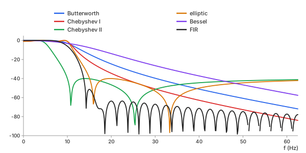
Chart 2. Gain of the six designs, low-pass at 10 Hz
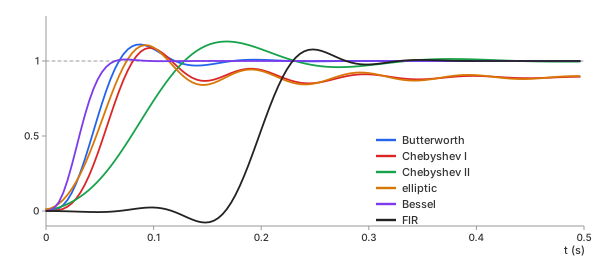
Chart 3. Step response of each design, one pass
| method | gain at 2 Hz | gain at 50 Hz | overshoot | delay at 2 Hz | error left |
|---|---|---|---|---|---|
| no filter | 1 | 0 dB | — | 0 | 0.367 |
| Butterworth | 1.0000 | −60.8 dB | 11.0% | 42 ms | 0.028 |
| Chebyshev I | 0.9427 | −72.7 dB | 22.0% | 46 ms | 0.082 |
| Chebyshev II | 0.9998 | −42.3 dB | 13.0% | 75 ms | 0.020 |
| elliptic | 0.9319 | −44.5 dB | 24.1% | 38 ms | 0.096 |
| Bessel | 0.9874 | −46.7 dB | 1.0% | 34 ms | 0.029 |
| FIR | 1.0043 | −74.7 dB | 7.7% | 201 ms | 0.029 |
Table 2. The six designs on the example. Delay: one pass. Error left: RMS against the true 2 Hz wave after zero-phase filtering, ends excluded
Every design reduces the error from 0.367 to below 0.1. The two filters with passband ripple, Chebyshev I and elliptic, leave the most residual error: at 2 Hz, they reduce the wave amplitude by 6–7%, reflecting the passband ripple specified in Math 6. The other four agree within 0.01.
In summary:
- Butterworth: the default choice; a flat passband and a predictable transition
- Chebyshev I: when a sharper transition matters more than preserving the exact passband amplitude
- Chebyshev II: when the stopband needs a guaranteed attenuation level and the passband must stay flat
- Elliptic: when the filter order must be as low as possible for a narrow transition
- Bessel: when preserving the shape of pulses and steps matters, as in timing signals or ECG morphology
- FIR: when exact linear phase or guaranteed stability matters, and a long filter is affordable
The basic calculator runs Butterworth filters in your browser. The advanced calculator offers all six designs, computed on the server.
Key Ideas
A filter is fully described by its response. These six ideas determine whether that response does what you want.
Cutoff and Order: The −3 dB Point and the Roll-Off
Cutoff $f_c$ is where the gain has dropped to $1/\sqrt{2} = 0.7071$, or −3 dB—half the power. Order $n$ sets the roll-off: well past the cutoff, the gain falls by $20n$ dB for every tenfold increase in frequency (Chart 4).
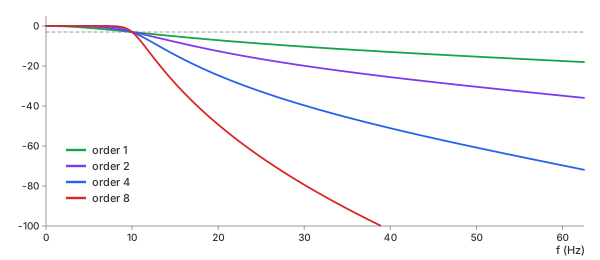
Chart 4. Butterworth low-pass at 10 Hz, order 1, 2, 4 and 8
| order | roll-off | gain at 50 Hz | step overshoot | sections |
|---|---|---|---|---|
| 1 | −20 dB/decade | −15.3 dB | 0.0% | 1 |
| 2 | −40 dB/decade | −30.4 dB | 4.4% | 1 |
| 4 | −80 dB/decade | −60.8 dB | 11.0% | 2 |
| 8 | −160 dB/decade | −121.6 dB | 16.5% | 4 |
Table 3. Order against attenuation and ringing
Doubling the order doubles the roll-off in decibels per decade. A higher order is not free: the edge gets sharper, but the filter generally produces more ringing and overshoot after sudden changes.
Phase Lag: Why Zero-Phase Filtering Needs the Whole Record
Causal filtering runs once, forward in time, using only past samples—the requirement for a real-time system. A causal filter generally delays the signal. The delay at a given frequency is the group delay $\tau(f)$; for the order-4 Butterworth filter at 2 Hz, it is 42.1 ms (Chart 5, red).
Zero-phase filtering runs the same filter forward and then backward over the result. The backward pass exactly cancels the phase shift introduced by the forward pass, while the gain is applied twice (Math 11).
Math 11.
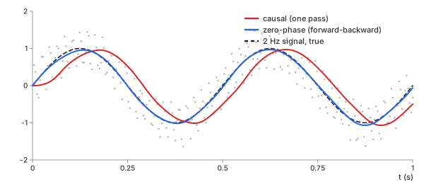
Chart 5. Causal and zero-phase Butterworth, order 4, 10 Hz, on the example
| filtering | delay at 2 Hz | error against the wave | error against the wave, delayed |
|---|---|---|---|
| causal | 42.3 ms | 0.369 | 0.028 |
| zero-phase | 1.5 ms | 0.028 | — |
Table 4. Measured delay and RMS error, ends excluded
The causal output is just as clean: its error drops to 0.028 once the 42 ms delay is taken into account. But it is late. When compared at the same instant, its error is 0.369—about as large as the error of the unfiltered data. Zero-phase filtering removes the delay: the measured residual delay of 1.5 ms is less than one sample (4 ms).
The cost is that the backward pass needs samples from the future, so zero-phase filtering works only on recorded data, never in real time. The gain is squared as well, so the original cutoff becomes the −6 dB point, and an order-4 filter has the same asymptotic roll-off as an order-8 filter.
The Moving Average Is a Low-Pass Filter, a Poor One
An $m$-point moving average is an FIR filter with $m$ equal weights. Its gain has a closed-form expression (Math 12).
Math 12.
An 11-point average at $f_s = 250$ Hz falls to −3 dB at 10.10 Hz—nearly the cutoff of the example. Chart 6 compares it with an order-4 Butterworth filter having exactly the same −3 dB point.
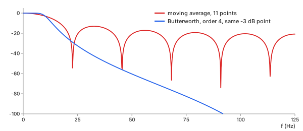
Chart 6. An 11-point moving average and a Butterworth filter with the same −3 dB point
| filter | −3 dB point | gain at 50 Hz | highest gain past 22.7 Hz |
|---|---|---|---|
| moving average, 11 points | 10.10 Hz | −20.8 dB | −13.0 dB |
| Butterworth, order 4 | 10.10 Hz | −60.4 dB | −29.0 dB |
Table 5. The same −3 dB point, very different stopbands
The moving average's gain falls to zero at multiples of $f_s / m = 22.7$ Hz, then rises again between them into sidelobes. At their worst, the sidelobes let 22% of the input amplitude through (−13 dB). At 50 Hz, the moving average lets 9% of the hum through—95 times as much as the Butterworth filter. A moving average is excellent at what smoothing asks of it: it is simple and produces no overshoot. But as a filter, it has no useful stopband.
Ripple Against Sharpness
Passband ripple is the wobble in gain below the cutoff. Chart 7 zooms in on the passband of the five feedback designs.
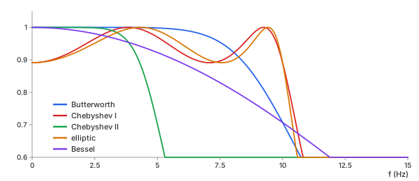
Chart 7. Passband gain of the five feedback designs, low-pass at 10 Hz
Chebyshev I and elliptic keep their gain between 0.8913 and 1 all the way to 10 Hz, then drop the fastest. Butterworth stays at 1 longer, then bends down to 0.7071 at 10 Hz. Bessel starts to droop immediately. No design can be both flat and steep: the ripple is what pays for the sharper edge.
Edges: The Start-Up Transient
A causal filter starts from rest, as if the signal had been zero before the first sample. Its output needs a few time constants to catch up: in Chart 5, the red curve starts at 0 and lags behind. For the FIR design, this start-up transient lasts a full 200 ms.
Zero-phase filtering with scipy.signal.sosfiltfilt—and in both calculators
here—reduces edge effects by extending the record at both ends before filtering. It pads
each end by $3(2s + 1)$ samples, where $s$ is the number of second-order sections, using
an odd reflection of the data. Each pass starts in the steady state corresponding to the
first or last value. For an order-4 filter, that is 15 samples, or 60 ms. In the first
0.1 s of the example, the zero-phase output has an RMS error of 0.048, compared with 0.028
in the interior.
The record must be longer than the padding. A record with fewer than 16 samples cannot be filtered with zero phase at order 4, so the calculators reject it and report the reason.
Nyquist: A Filter Cannot Undo Aliasing
A sampled signal can represent frequencies only up to the Nyquist frequency, $f_s / 2$. A cutoff above it is not meaningful for the sampled data, and both calculators reject one. Anything above $f_s / 2$ before sampling does not simply disappear: it folds down to a lower frequency, an effect called aliasing.
Chart 8 samples a 200 Hz tone at 250 Hz. The resulting samples are exactly the same as those of a 50 Hz tone with a 180° phase reversal.
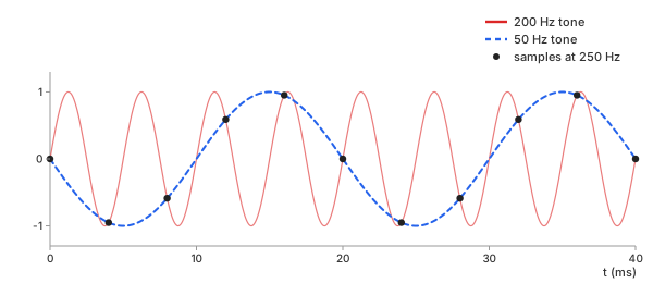
Chart 8. A 200 Hz tone sampled at 250 Hz lands on 50 Hz
No digital filter can distinguish this alias from a real 50 Hz hum: in the sampled data, they are identical. The only way to prevent this is to use an analog low-pass filter before the analog-to-digital converter. The Fourier transform page shows where an alias appears in the spectrum.
Filter in hertz, check the response, and sample fast enough first.
REFs
SciPy scipy.signal.butter SciPy scipy.signal.sosfiltfilt SciPy scipy.signal.firwin Wikipedia, Butterworth filter Wikipedia, Chebyshev filter Wikipedia, Elliptic filter Wikipedia, Bessel filter Wikipedia, Finite impulse response Smoothing Methods: Moving Average, EWMA, Savitzky-Golay, Gaussian, Median Fourier Transform (DFT, FFT): What Frequencies Are in My Data? Detrending & Baseline Correction: How to Remove Drift from Measured Data