Smoothing Methods: Moving Average, EWMA, Savitzky-Golay, Gaussian, Median

Six ways to pull noise out of a signal without passing through every point - moving average, EWMA, Savitzky-Golay, Gaussian, median, and smoothing splines - and the trade-off none of them can remove.

What is smoothing, and when you want it instead of interpolation

Suppose you measured a signal and it looks like this:

x = 0  1  2  3  4  5  6  7  8  9
y = 2  6  1  7  3  8  2  9  4  10

There is probably a real trend hiding in there - rising, say - buried under noise that has nothing to do with what you actually care about: a sensor's jitter, rounding error, a shaky measurement. You do not want a curve that hits every one of those ten points exactly. You want a curve that ignores the jitter and shows the trend.

That is smoothing: build a new value at (or near) every point by combining it with its neighbors, on purpose losing some detail so noise cancels out.

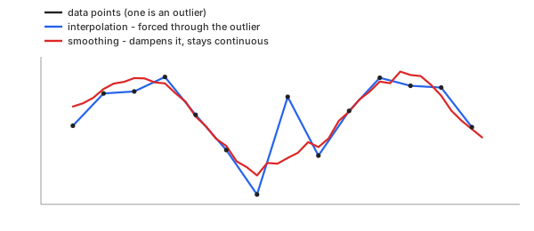
Smoothing is interpolation's opposite number, not its cousin. Interpolation passes through every point exactly - it is exact at the data, by definition. Smoothing deliberately misses points; that is the only way it can reject noise. If you asked interpolation to "smooth" your data it would still draw a curve through every noisy wiggle, because passing through the data is the one thing it is not allowed to give up.

So: if you trust every number you measured and want the value between two of them, you want interpolation. If you do not fully trust the numbers you measured and want the value near one of them with the noise reduced, you want this page.

Noisy data with one outlier: interpolation is forced to spike to the bad value, smoothing dampens it and stays continuous

Methods

Every method below answers the same question - "what do I do with a point's neighbors?" - differently. Six are built into the advanced calculator; a seventh, LOESS, is explained here for completeness but not offered there yet (see the note at the end of that section).

The same noisy data smoothed by moving average, Savitzky-Golay and median at once

Moving average (simple, centred)

In plain words. At each point, look at a fixed number of neighbors on both sides - the window - and replace the point with their plain average.

Control parameters. window ($k$ below, where window $=2k+1$) - how many neighbors on each side get averaged in.

Basic idea. For a window of $2k+1$ points centred on index $i$:

$$\text{smoothed}_i = \frac{1}{2k+1}\sum_{j=-k}^{k} y_{i+j} = \frac{1}{2k+1}\left(y_{i-k} + \dots + y_i + \dots + y_{i+k}\right)$$

$$\begin{aligned}\text{smoothed}_i &= \frac{1}{2k+1}\sum_{j=-k}^{k} y_{i+j} \\ &= \frac{1}{2k+1}\left(y_{i-k} + \dots + y_i + \dots + y_{i+k}\right)\end{aligned}$$

Slide that window across every point and you get the whole smoothed series.

Important characteristics. It is a straight, unweighted mean - every neighbor counts exactly as much as every other, near or far. That is also its whole weakness: a single wild outlier in the window pulls the average toward itself for every point whose window includes it, smearing the outlier's influence across $2k+1$ output points instead of containing it to one.

Advantages

Simplest method here, cheapest to compute
Easy to explain to someone who has never heard the word "filter"
No overshoot: the output is always between the min and max of its window

Disadvantages

An outlier smears across the whole window instead of staying local
Sharp features (a real step, a real peak) get rounded off along with the noise
No control over how much weight nearby vs. far points get - they are all equal

A moving average at window 3, 9, and 21 - wider windows smooth more but lag more

Exponential moving average (EWMA)

In plain words. Instead of a fixed window, keep a running average that leans on the newest point a bit and on yesterday's running average a lot. Old points never fully leave, they just fade.

Control parameters. alpha ($\alpha$ below) - how much weight the newest point gets over the running average so far (span sets this same $\alpha$ indirectly, not a second knob).

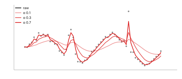
Basic idea. One number, $\alpha$ between 0 and 1, controls the fade:

$$\text{smoothed}_0 = y_0,\qquad \text{smoothed}_i = \alpha\, y_i + (1-\alpha)\,\text{smoothed}_{i-1}$$

$$\begin{aligned}\text{smoothed}_0 &= y_0 \\ \text{smoothed}_i &= \alpha\, y_i + (1-\alpha)\,\text{smoothed}_{i-1}\end{aligned}$$

A bigger $\alpha$ trusts the newest point more and fades faster; a smaller one remembers longer. $\alpha$ is sometimes given indirectly as a span $N$, converted by $\alpha = 2 / (N + 1)$ - the two knobs are the same knob wearing a different label.

Important characteristics. Unlike every other method here, EWMA is naturally causal: $\text{smoothed}_i$ only ever depends on points up to and including $i$, never on anything after it. That makes it the natural choice for a live stream, where "after" does not exist yet - and it is also why it lags, which the phase-lag section below is about.

Advantages

Works on a live stream - no need to wait for future points
One parameter, and it has an intuitive "how much memory" reading
Cheap: one multiply-add per new point, no window to store

Disadvantages

Always lags the true signal - see phase lag, below
An outlier still leaks into every following point, just with decaying weight
Not centred, so it answers a slightly different question than the others

An exponential moving average at α 0.1, 0.3, and 0.7 - higher α tracks the signal more closely

Savitzky-Golay

In plain words. Instead of averaging the window, fit a low-degree polynomial (a line, a parabola, a cubic) through it by least squares, then read off that polynomial's value at the centre point.

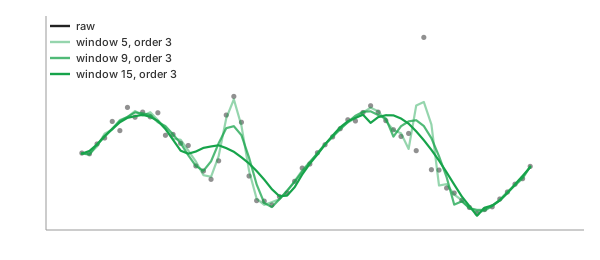
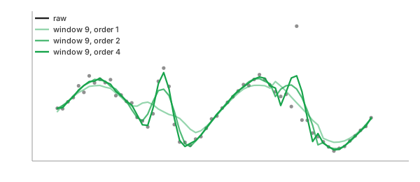
Control parameters. window ($2k+1$ points, same as above) sets the neighborhood size; order ($p$ below) sets the fitted polynomial's degree - the only method here with two independent knobs, hence two figures below instead of one.

Basic idea. For a window of $2k+1$ points around index $i$, solve for the polynomial of degree $p$ that best fits those points in the least-squares sense:

$$p(x) = c_0 + c_1 x + c_2 x^2 + \dots + c_p x^p$$

then use that polynomial's value at $i$ as the smoothed output. Slide the window and refit at every point (in practice this reduces to one fixed set of weights per position once the window and degree are fixed, which is the trick that makes it fast - but "fit and evaluate" is what it does).

Important characteristics. A moving average is a Savitzky-Golay filter with degree 0 - a flat line is the least-squares best fit of a constant to the window, which is just the mean. Raising the degree lets the filter track a genuine peak or a genuine slope in the data instead of flattening it, which is exactly what a plain average cannot do. The classic use case is a real spectral peak: a moving average blunts it, Savitzky-Golay with degree 2 or 3 preserves its height and width far better for the same amount of noise rejected.

Advantages

Preserves peak height and width much better than a moving average
Degree 0 is a moving average, so it is a strict generalization, never worse
Well understood, the standard choice in spectroscopy and chromatography

Disadvantages

Two knobs to choose (window and degree) instead of one
Degree must stay below the window size, or the fit is not defined
Still a linear filter - a single spike still smears, just less than a plain average

A Savitzky-Golay filter at window 5, 9, and 15, order fixed at 3 - wider windows smooth more

A Savitzky-Golay filter at order 1, 2, and 4, window fixed at 9 - higher order tracks peaks more closely

Gaussian kernel

In plain words. Average the window like a moving average, but let nearby points count more and far points count less, fading smoothly by distance instead of cutting off sharply at the window edge.

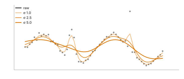
Control parameters. sigma ($\sigma$ below) - how quickly a neighbor's weight fades with its distance from the centre.

Basic idea. Each neighbor at offset $d$ from the centre gets a weight from the bell curve, then the weights are normalized so they still sum to 1:

$$w(d) = \exp\!\left(-\frac{d^2}{2\sigma^2}\right),\qquad r = \lceil 3\sigma \rceil$$

$$\text{smoothed}_i = \frac{\sum_{d=-r}^{r} w(d)\,y_{i+d}}{\sum_{d=-r}^{r} w(d)} = \frac{w(-r)\,y_{i-r} + \dots + w(0)\,y_i + \dots + w(r)\,y_{i+r}}{w(-r) + \dots + w(0) + \dots + w(r)}$$

$$\begin{aligned}\text{smoothed}_i &= \frac{\sum_{d=-r}^{r} w(d)\,y_{i+d}}{\sum_{d=-r}^{r} w(d)} \\ &= \frac{w(-r)\,y_{i-r} + \dots + w(0)\,y_i + \dots + w(r)\,y_{i+r}}{w(-r) + \dots + w(0) + \dots + w(r)}\end{aligned}$$

The window stops at $r$ neighbors each side: beyond three sigmas the weights are negligible, and the calculator does not compute them.

$\sigma$ controls how fast the weight fades - a small $\sigma$ barely looks past its immediate neighbors, a large one behaves almost like a wide moving average.

Important characteristics. A moving average gives a window's nearest and farthest point equal say, which shows up as small step-like artifacts as the window slides. A Gaussian kernel's weights are smooth, so the output has no such steps - it is the smoothest-looking of the simple averaging methods, at the cost of a less intuitive knob than "how many points."

Advantages

Smoother-looking output than an equal-weight moving average
One continuous knob ($\sigma$) instead of a hard window-size cutoff
Well studied, standard in image and signal processing

Disadvantages

Still linear, so a spike still smears across the effective window
Sigma is less intuitive to pick than "how many neighbors"
Needs evenly spaced x, like the moving average and Savitzky-Golay above

A Gaussian-weighted moving average at σ 1, 2.5, and 5 - a wider kernel smooths more

Median filter

In plain words. Instead of averaging the window, sort it and take the middle value.

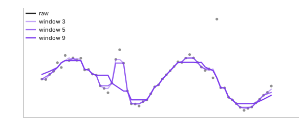
Control parameters. window ($k$ below, where window $=2k+1$) - how many neighbors are sorted before picking the middle one.

Basic idea.

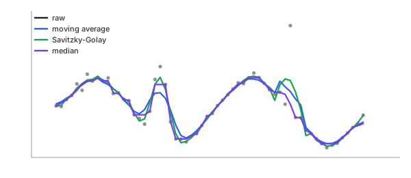
$$\text{smoothed}_i = \operatorname{median}(y_{i-k}, \dots, y_i, \dots, y_{i+k})$$

Important characteristics. This is the odd one out on this list, and the whole reason it is here: every method above is linear - the output is some weighted sum of the window's values - and a linear filter cannot help but smear a single huge outlier across its whole window, because the outlier still enters the sum with some nonzero weight. The median is non-linear. A single spike, no matter how large, is just one value among $2k+1$; sort it, and it lands at one end, contributing to the middle value only if the window is mostly spikes. One real outlier among real neighbors gets thrown out entirely, not smeared - the median simply never picks it.

That is the one property that earns the median a place on this list even though it "smooths" worse than the others by most measures: a real, otherwise-smooth signal with one bad sample comes back clean, where every linear method above leaves a dent centred on the bad sample.

To flag the bad sample rather than smooth it away, add a band around this median: that is the Hampel filter, one of the methods in Outlier Detection.

Advantages

Rejects a single outlier completely instead of smearing it
Preserves sharp edges (a real step) far better than any linear filter
No overshoot: the output is always one of the values already in the window

Disadvantages

Not linear, so it has no simple frequency-response description
Flattens genuine narrow peaks the way a moving average does, spikes aside
Slower to compute than a running sum (has to sort, or maintain a sorted structure)

A median filter at window 3, 5, and 9 - wider windows smooth more but need more real neighbors

LOESS / LOWESS

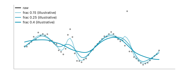
In plain words. Like Savitzky-Golay - fit a low-degree polynomial in a local window and evaluate it at the centre - but weight the points in that window by distance (like the Gaussian kernel does) and, in its usual form, re-weight down whatever points looked like outliers on a first pass and refit.

Control parameters. frac ($r$ below) - what share of the data counts as "nearby" for each point's local fit.

Basic idea. For each point, take the nearest fraction $r$ of the data (a "span," e.g. $r=0.3$), fit a weighted low-degree polynomial where closer points count more, evaluate at the centre, and optionally iterate: down-weight points with large residuals and refit, which is what makes it robust to outliers the way the median is.

Important characteristics. LOESS combines Savitzky-Golay's local-polynomial idea with the Gaussian kernel's distance weighting and (with robust iterations) some of the median's outlier resistance - which makes it the most flexible method on this list, and the most expensive to compute.

Advantages

No assumption about the shape of the underlying trend
Robust iterations give it real outlier resistance, unlike a plain weighted average
Widely used for exploratory data analysis and scatterplot trend lines

Disadvantages

Two or more knobs (span, degree, robustness iterations) instead of one
Expensive: a separate weighted fit at every output point
Not offered on this site's advanced calculator yet - it needs a Python library (statsmodels) this site's backend does not currently ship, to avoid adding a new dependency without it being a deliberate, separate decision

$A LOWESS fit at frac 0.15, 0.25, and 0.4, illustrative only - not offered on the calculator yet$

Smoothing spline (penalised)

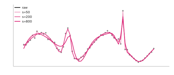
In plain words. Instead of a local window at all, fit one curve to the whole series at once, balancing two competing goals: stay close to the data, and stay smooth (avoid wiggling). A single knob decides how much either goal wins.

Control parameters. s - a residual-error budget: a larger s allows more error, which is the same trade-off as "penalty" below, approached from the other direction.

Basic idea. Find the curve $f$ that minimizes:

$$\sum_{i=1}^{n} \big(y_i - f(x_i)\big)^2 + \text{penalty}\cdot\text{roughness}(f) = \big(y_1 - f(x_1)\big)^2 + \dots + \big(y_n - f(x_n)\big)^2 + \text{penalty}\cdot\text{roughness}(f)$$

$$\begin{aligned}&\sum_{i=1}^{n} \big(y_i - f(x_i)\big)^2 + \text{penalty}\cdot\text{roughness}(f) \\ &= \big(y_1 - f(x_1)\big)^2 + \dots + \big(y_n - f(x_n)\big)^2 + \text{penalty}\cdot\text{roughness}(f)\end{aligned}$$

where $n$ is the number of data points and $\text{roughness}(f)$ grows with how much the curve bends. A tiny penalty lets the curve chase the data closely (approaching interpolation); a large one flattens it toward a straight line. This site's calculator exposes the same idea from the other direction, as scipy does: a smoothing factor s that caps how much total squared error the fit is allowed before it is forced to add curvature to reduce it further.

When you want an equation with a few coefficients instead of one smoothed value per point, that is Curve Fitting.

Important characteristics. Because it is a single global fit rather than a sliding window, a smoothing spline has no window to shrink at an edge the way every window-based method above does - the edge is just wherever the one curve happens to end. That is a genuine advantage over a window-based method when the edge behavior matters.

Advantages

One global, smooth curve - useful when you want to evaluate it anywhere, not just at the data points
No separate edge rule needed - the fit is global, not windowed
Closely related to cubic spline interpolation, familiar if you have read that page

Disadvantages

The smoothing factor is not as intuitive to pick as "how many neighbors"
A global fit: one bad region of the data can influence the curve elsewhere
More expensive than a sliding window over the same data

A smoothing spline at s=50, 200, and 800 - larger s trades closeness to the data for smoothness

Which one should you pick

If your data is...	use
evenly spaced, no outliers, you just want it simple	moving average
a live stream, arriving one point at a time	EWMA
has real peaks you must not blunt	Savitzky-Golay
wants the smoothest-looking curve, no hard cutoff	Gaussian kernel
has occasional spikes or dropouts you want gone, not smeared	median filter
unevenly spaced, and you want a full curve, not just point values	smoothing spline

None of these is more correct than the others - they are bets about which kind of imperfection in your data matters most. Pick the failure you can live with.

The one knob: window size, and the trade it makes

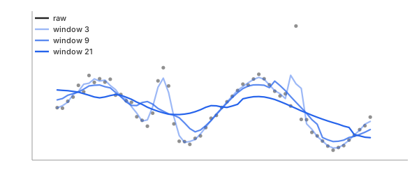
Every window-based method above has one knob that matters most: how many neighbors to include. Make it small and the noise survives almost untouched - you have barely averaged anything. Make it large and the real signal flattens along with the noise - eventually a wide enough moving average just returns a flat line near the series' overall mean.

There is no window size that avoids this. A smaller window leaves more noise in (higher variance from one sample to the next); a larger window distorts the true shape more (higher bias, systematically off from the real signal). This is the bias-variance trade, and it is not a bug to be fixed - it is the actual content of "how much should I smooth," and every method on this page, no matter how clever, only moves where that trade sits. None of them removes it.

Savitzky-Golay's polynomial degree, the Gaussian kernel's $\sigma$, and the smoothing spline's penalty are all the same knob wearing a different name: more flexibility (a higher degree, a larger $\sigma$, a smaller penalty) tracks the data more closely and removes less noise; less flexibility does the opposite.

Edges: every method has to invent data at the first and last half-window

A centred window at the very first point wants neighbors before the start of the data. They do not exist. Every smoothing implementation has to decide what to do there, and the common choices are all a little dishonest: reflect the data back across the edge as if it were a mirror, repeat the edge value outward as if the signal were flat before it started, or wrap around as if the series were periodic. All three invent numbers nobody measured.

This site's calculators do none of them. The window shrinks near an edge instead: the point one step from the start is smoothed from whatever real neighbors actually exist on both sides of it, and the first point itself is smoothed from only the real points after it, using a full window wherever one fits and a shrunk one wherever it does not. That is a smaller sample at the edges - the edge values are noisier than the interior ones - but every number that goes into an edge value was actually measured. Nothing here reflects, repeats, or wraps.

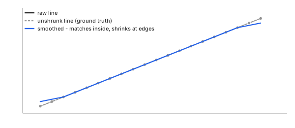
A perfectly straight line smoothed by a moving average: exact in the interior, shifted at the shrunk edges

One consequence worth predicting before you see it in the calculator: a moving average does not reproduce a straight line at the edges, even though it reproduces one exactly in the interior. In the interior, a symmetric window around a point on a line averages to that point's own value by symmetry. Near an edge the shrunk window is no longer symmetric, so the average is pulled toward whichever side has more points - the line's edge value comes back shifted. Savitzky-Golay with degree 1 or higher does not have this problem: a least-squares line fit through any subset of points that are already exactly collinear reproduces that line exactly, shrunk window or not, because there is zero error left to correct no matter how few points the fit sees. The calculator's own fixture data is built to show exactly this difference.

Phase lag: a causal filter shifts the curve right, a centred one does not

Every method above except EWMA is centred: smoothing point $i$ uses points both before and after it, so a real feature (a step, a peak) in the output lands at the same $x$ where it happened in the input.

EWMA is causal: smoothing point $i$ only uses points up to and including $i$, because that is what a live stream can offer - the future has not arrived yet. The unavoidable cost is phase lag: a real step in the underlying signal shows up in the EWMA output only after the running average has had time to catch up to it, which means it appears to happen later than it really did, and a real peak in the input reads a little lower and a little later in the causal output than it should.

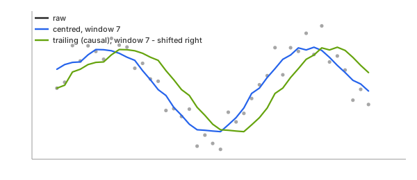
A trailing (causal) average shifted right compared to a centred moving average on the same data

This is not a flaw to fix - EWMA is not "worse" than a centred filter, it answers a different question. If you are watching a live sensor and need this instant's best guess with no access to the future, a lag is the price of admission and a centred method is not an option at all: it needs data from after "now," which does not exist yet on a live stream.

Smoothing is low-pass filtering. Every linear method above keeps the slow part of a signal and removes the fast part - a low-pass filter set in points instead of hertz. See how a moving average compares with a designed filter, and how forward-backward filtering removes the lag, in Digital Filters: the moving average is a low-pass filter.

Linear vs non-linear, and why it matters for spikes

Moving average, EWMA, Savitzky-Golay, the Gaussian kernel, and the smoothing spline are all linear filters: every output value is some weighted sum of input values, with the weights fixed in advance and not depending on what the data actually looks like. That has a specific, unavoidable consequence: a single huge outlier is still in that sum with some nonzero weight, so it still pulls every output point whose window includes it - it gets smeared across the window, not removed.

The median filter is non-linear: sorting and taking the middle value is not a weighted sum at all, and a value's influence on the output does not grow with its size. A single spike that is far larger than its neighbors simply never becomes the middle value once the window is sorted - the filter deletes it instead of diluting it. That single property, not raw smoothing power, is the entire reason the median filter earns a place on this list next to five methods that are individually smoother-looking on clean data.

REFs

Scipy savgol_filter Savitzky & Golay (1964), "Smoothing and Differentiation of Data by Simplified Least Squares Procedures" Scipy gaussian_filter1d Scipy medfilt Scipy UnivariateSpline NIST Engineering Statistics Handbook: EWMA control charts Cleveland (1979), "Robust Locally Weighted Regression and Smoothing Scatterplots" (LOWESS) statsmodels lowess