How to bring a drifting signal back to a flat zero baseline (baseline correction, leveling, or zeroing): mean removal, linear detrending, polynomial baseline fitting, and asymmetric least squares (ALS) — and why ordinary least-squares fitting fails when peaks are present.
Contents
What Is Detrending? What Does the Signal Look Like After the Drift Is Removed?
A measurement rarely sits at zero. A spectrometer's background rises with wavelength, a sensor warms up and drifts over an hour, and a chromatogram rides on a slowly changing solvent signal. The features you want to study—peaks, oscillations, and events—sit on top of a slowly varying curve that is unrelated to them. This slow curve is called the baseline or trend.
Detrending, also called baseline correction—leveling or flattening when correcting a measured surface, and zeroing when establishing a true zero reference—estimates this baseline and subtracts it from the original signal. The residual signal is then centered around a flat zero baseline (Fig 1):
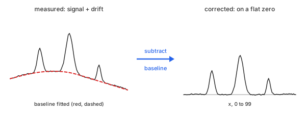
Fig 1. Fit a baseline under the data, subtract it, and the peaks stand on zero
Every method on this page follows the same two steps. The only difference is how the baseline $b$ is estimated (Math 1):
Math 1.
Here, $y_i$ is the measured value at $x_i$, $b(x_i)$ is the baseline at that point, $d_i$ is the detrended value, and $N$ is the number of data points.
Detrending is not smoothing: smoothing removes high-frequency noise while preserving the slow trend; detrending removes the slow trend while retaining everything else, including noise.
Consider an example with 100 data points, from $x = 0$ to $x = 99$. Three peaks, with heights of 3, 5, and 2, are located at $x = 25$, 50, and 75, respectively. They sit on a baseline that rises, bends, and falls—a combination of a quadratic curve and a slow wave—with a little noise added.
Because the data is synthetic, the true baseline is known. This allows each method to be evaluated against it (Table 1).
| x | y (measured) | true baseline |
|---|---|---|
| 0 | 2.0001 | 2.0000 |
| 10 | 2.4845 | 2.4600 |
| 25 | 5.8770 | 2.8864 |
| 40 | 2.9313 | 2.9064 |
| 50 | 7.7381 | 2.7000 |
| 60 | 2.3895 | 2.3600 |
| 75 | 3.7516 | 1.7172 |
| 90 | 1.0588 | 1.0600 |
| 99 | 0.5914 | 0.6932 |
Table 1. The example: 9 of its 100 points, with the true baseline under each
The bold row, $x = 50$, corresponds to the top of the tallest peak. Each method below is worked out by hand at that point. Chart 1 plots all 100 data points.
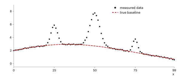
Chart 1. The example: measured data and the true baseline under it
The task: find the dashed baseline using only the data points.
Methods
Four ways to estimate the baseline $b$, from the simplest to the method designed for signals with peaks. The first three use least-squares fitting: they fit a curve as closely as possible to all the data points, subject to the chosen model's shape. The fourth treats points above and below the baseline differently.
Mean Removal
In plain words. Calculate the average of all the measured values and subtract it from each one. The resulting data is centered around zero.
Basic idea. Assume the baseline is a single constant equal to the mean $\bar{y}$ (Math 2).
Math 2.
Example. At $x = 50$ (Math 3):
Math 3.
Important characteristics. A flat line cannot follow a slope or a curve. Mean removal centers the data around zero, but does nothing beyond that.
Advantages
- No parameters to choose or tune
- Removes the mean component, which eliminates the 0 Hz (DC) component in an FFT
Disadvantages
- Any slope or curvature remains in the detrended signal
- Peaks raise the mean, shifting the zero baseline below the true baseline
Linear Detrending
In plain words. Draw the straight line that fits all the data points as closely as possible, then subtract it from the data.
Basic idea. Model the baseline as a straight line, $b(x) = \beta_0 + \beta_1 x$, where the slope $\beta_1$ and the intercept $\beta_0$ are chosen to minimize the sum of squared differences between the measured values and the fitted line. This is the least-squares line (Math 4).
Math 4.
In the example. Calculate $\beta_1$ and $\beta_0$ using two sums over all 100 data points, with $\bar{x} = 49.5$ and $\bar{y} = 2.8045$ (Math 5):
Math 5.
Then calculate the baseline at $x = 50$ and subtract it from the measured value to obtain the detrended value (Math 6):
Math 6.
Important characteristics. Removes both a constant offset and a steady
linear trend. This is what
scipy.signal.detrend
does by default.
Advantages
- A single formula with no tuning parameters
- Works with any spacing between data points
- A standard preprocessing step before applying an FFT to a drifting signal
Disadvantages
- A curved baseline leaves a bow-shaped residual in the detrended signal
- Peaks pull the fitted line toward themselves, just as they do with mean removal
Polynomial Baseline
In plain words. Use the same approach as linear detrending, but allow the baseline to bend: fit a smooth polynomial curve of a chosen order to the data, then subtract it.
Basic idea. Model the baseline as a polynomial of order $m$, fitted by least squares. First, scale $x$ to the interval $s \in [-1, 1]$ so that higher powers remain on a similar numerical scale and the fit is better conditioned (Math 7).
Math 7.
An order-1 polynomial is equivalent to linear detrending. In the example, consider an order-3 polynomial evaluated at $x = 50$ (Math 8).
Math 8.
The true baseline at this point is 2.7000 (Table 1). The cubic fit lies 1.1 units above it: the three peaks have pulled the curve upward, causing the tallest peak to lose one-fifth of its height after detrending.
Important characteristics. A polynomial can follow a curved baseline, to the extent allowed by its order. Choosing the polynomial order is the main decision, and it matters (see Polynomial Order).
Advantages
- Follows bends that a straight line cannot
- Works with any spacing between data points
- Fast: requires solving only a small least-squares problem
Disadvantages
- Peaks pull the fitted curve upward, and a flexible curve can extend into the peaks
- High-order polynomials can oscillate near the ends of the record
Asymmetric Least Squares (ALS)
In plain words. Fit a smooth curve, then identify which points lie above it and give them less weight because they are likely to be peaks. Fit the curve again using the updated weights, and repeat until the curve runs beneath the peaks rather than cutting through them.
Basic idea. Eilers and Boelens (2005) estimate the baseline $z$ by balancing two objectives: staying close to the data and maintaining smoothness. The method uses a Whittaker smoother with asymmetric weights. Closeness to the data is controlled by the weights $w_i$, while smoothness is enforced by penalizing the second differences $\Delta^2 z_i = z_{i+2} - 2 z_{i+1} + z_i$, scaled by $\lambda$ (Math 9).
Math 9.
The asymmetry comes from the weights: a point above the current baseline receives the small weight $p$, while a point below it receives the larger weight $1 - p$ (Math 10).
Math 10.
Each iteration requires solving a linear system, where $W$ is the diagonal weight matrix and $D$ is the second-difference matrix (Math 11).
Math 11.
Start with all weights set to 1, solve for the baseline, update the weights, and solve again. In this example, use 10 iterations, $\lambda = 10^3$, and $p = 0.01$. At $x = 50$ (Math 12):
Math 12.
The estimated baseline is only 0.08 above the true baseline, and the peak retains its full height after correction.
Important characteristics. The system matrix is banded, making each solve efficient even for long records. The second-difference penalty assumes evenly spaced data points.
Advantages
- Stays beneath peaks instead of cutting through them
- Follows a wide range of smooth baseline shapes without requiring a polynomial order
Disadvantages
- Requires tuning two parameters, $\lambda$ and $p$, for each type of data
- Requires evenly spaced data points
- Assumes peaks rise above the baseline; downward dips may be mistaken for the baseline
Which One Should You Choose?
Chart 2 overlays the four estimated baselines on the example signal. Table 2 compares each estimate with the true baseline and shows the height of each peak after correction.
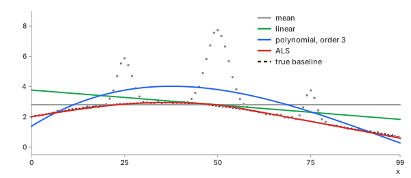
Chart 2. Four baselines on the example; the true one dotted
| method | error RMS | error max | peak 25 | peak 50 | peak 75 |
|---|---|---|---|---|---|
| true baseline | 0 | 0 | 2.991 | 5.038 | 2.034 |
| mean | 0.900 | 2.111 | 3.073 | 4.934 | 0.947 |
| linear | 0.739 | 1.774 | 2.593 | 4.943 | 1.446 |
| polynomial, order 3 | 0.770 | 1.121 | 2.113 | 3.934 | 1.415 |
| ALS | 0.049 | 0.099 | 3.036 | 4.957 | 2.053 |
Table 2. Baseline error against the truth, and the peak heights each method leaves
The least-squares methods have an average error of 0.7 to 0.9. Mean removal and linear detrending happen to give values close to the true baseline at $x = 50$, but their errors reach 2 elsewhere. With mean removal, the peak at $x = 75$ loses half its height.
Only ALS preserves all three peaks.
In summary:
- Mean removal: when only a constant offset needs to be removed, such as before an FFT
- Linear detrending: for steady drift without large peaks, such as sensor creep or a time series prepared for an FFT
- Polynomial baseline: for a curved background with small or few peaks, including data with unevenly spaced points
- ALS: for peaks on a curved background, such as spectra and chromatograms
The basic calculator runs mean removal, linear detrending, and polynomial fitting in your browser. The advanced calculator also supports ALS, which is computed on the server.
Key Ideas
Subtraction itself is exact. Everything depends on the baseline estimate—and there are four ways to get it wrong.
Polynomial Order: Too Low Leaves a Trend; Too High Eats the Peaks
Polynomial order $m$ is the highest power in Math 7. It determines how much the baseline can bend. Chart 3 fits the example using three different polynomial orders.
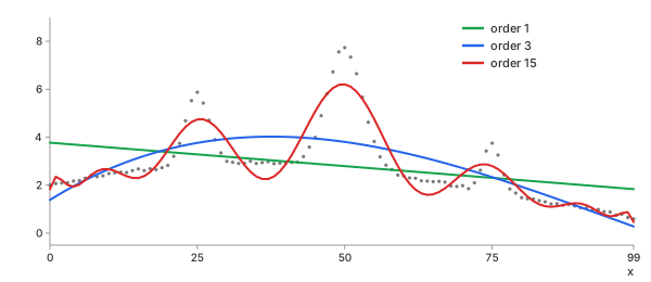
Chart 3. Polynomial baselines of order 1, 3 and 15 on the example
| order | error RMS | peak 50 left |
|---|---|---|
| 1 | 0.739 | 4.943 |
| 3 | 0.770 | 3.934 |
| 15 | 1.214 | 1.532 |
Table 3. Error and the height left at the tallest peak (true 5.038), by order
Order 1 cannot bend, so the curvature of the true baseline remains in the detrended signal. Order 15 is flexible enough to follow the peaks themselves, removing much of the tallest peak. When peaks are present, no polynomial order is ideal: increasing the order reduces the residual trend but also removes more of the signal.
Use a low order—typically 2 to 4—when the peaks are small relative to the overall signal. Use ALS when the peaks are more prominent.
Why Least Squares Is Pulled Up by Peaks
Least squares minimizes the sum of squared residuals, $\sum_i (y_i - b(x_i))^2$, giving every point the same weight. A peak consists of consecutive points far above the baseline, so the fit cannot ignore them. It moves upward toward the peaks to reduce their squared residuals. In Chart 2, the cubic fit lies 1.1 units above the true baseline at $x = 50$, while the mean baseline lies above the true baseline at both ends.
ALS changes only the weights. With $p = 0.01$, a point above the estimated baseline receives one ninety-ninth of the weight of a point below it (Math 10). As a result, peaks exert less upward influence, allowing the baseline to settle closer to the points between them.
ALS Parameters: λ for Stiffness, p for Asymmetry
Smoothness parameter $\lambda$ controls the trade-off between baseline smoothness and closeness to the data (Math 9). A small $\lambda$ allows the baseline to bend freely and climb into the peaks. A large $\lambda$ makes it stiffer, tending toward a straight line that may fail to follow the true curved baseline (Chart 4).
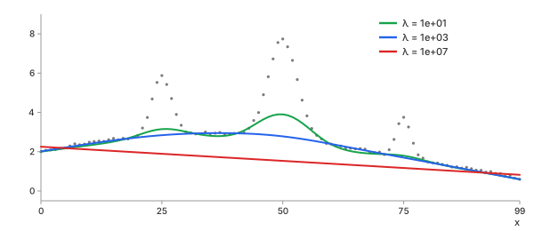
Chart 4. ALS with $\lambda = 10$, $10^3$, $10^7$; $p = 0.01$
Asymmetry parameter $p$ controls the weight of a point above the baseline (Math 10). At $p = 0.5$, points on both sides receive equal weights, producing an ordinary smooth fit that is pulled into the peaks. Smaller values of $p$ allow the fit to ignore the peaks more effectively (Chart 5).
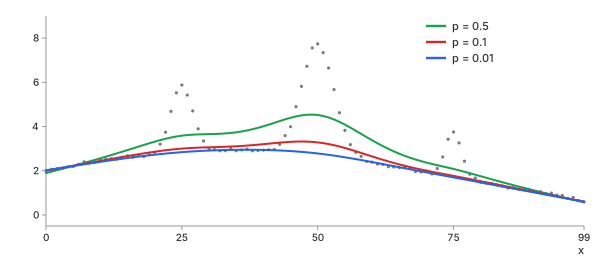
Chart 5. ALS with $p = 0.5$, 0.1, 0.01; $\lambda = 10^3$
| setting | error RMS | peak 50 left |
|---|---|---|
| $\lambda = 10$ | 0.362 | 3.836 |
| $\lambda = 10^3$, $p = 0.01$ | 0.049 | 4.957 |
| $\lambda = 10^7$ | 0.808 | 6.205 |
| $p = 0.5$ | 0.813 | 3.217 |
| $p = 0.1$ | 0.231 | 4.456 |
Table 4. ALS settings against the truth; tallest peak true 5.038
An overly stiff baseline can overshoot, too. At $\lambda = 10^7$, the nearly straight baseline runs below the curved baseline, causing the corrected peak to appear 1.2 units too tall. Eilers and Boelens suggest using $p$ between 0.001 and 0.1 and $\lambda$ between $10^2$ and $10^9$. The appropriate value of $\lambda$ depends on the number of data points and the width of the peaks. Tune the parameters visually on one record, then keep the same settings for all records of the same type.
Trend and the FFT: Drift Fills the Low-Frequency Bins
Drift in a spectrum — a Fourier transform interprets any slow trend as low-frequency content. Take the two tones from the Fourier transform page: a 1 Hz tone with an amplitude of 1.0 and a 3 Hz tone with an amplitude of 0.5, recorded for 8 seconds at 16 samples per second. Now add a drift of $1 + 0.5\,t$ (Chart 6).
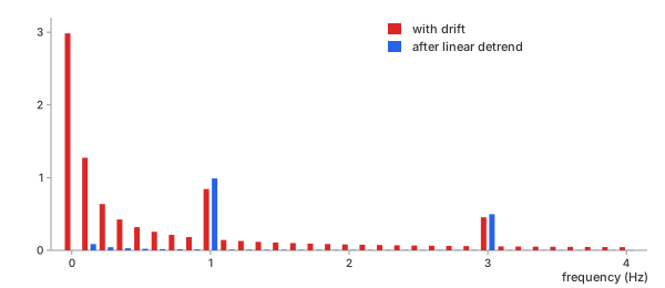
Chart 6. Spectrum of two tones plus a linear drift, before and after a linear detrend
| bin | with drift | after linear detrend |
|---|---|---|
| 0 Hz | 2.984 | 0.000 |
| 0.125 Hz | 1.273 | 0.086 |
| 1 Hz (true 1.0) | 0.843 | 0.989 |
| 3 Hz (true 0.5) | 0.454 | 0.497 |
Table 5. Amplitudes before and after detrending
The drift is not periodic. To the FFT, the end of the record must wrap back to its beginning, creating a discontinuity that causes spectral leakage across the frequency bins. The 0 Hz bin captures the offset, while the nearby bins show a decaying tail. The two tones' amplitudes are underestimated by 16% and 9%, respectively. A single linear detrend removes the tail and brings both amplitudes to within 2% of their true values.
Detrend first, then transform.
REFs
pybaselines, Whittaker baselines - asls, after P. H. C. Eilers, H. F. M. Boelens, Baseline Correction with Asymmetric Least Squares Smoothing, 2005 SciPy scipy.signal.detrend Wikipedia, Polynomial regression Fourier Transform (DFT, FFT): What Frequencies Are in My Data? Smoothing Methods: Moving Average, EWMA, Savitzky-Golay, Gaussian, Median