How cross-correlation finds the time delay between two signals and autocorrelation finds the period of one - starting from Pearson's r at lag 0, with normalization, significance and the FFT method.
Contents
What Is Cross-Correlation? How Far Apart Are Two Signals?
Two sensors often record the same event at different times. A microphone farther from a sound hears it later, a downstream flow meter sees a pressure pulse after the upstream one, and a seismometer far from an earthquake shakes after one close to it. The delay between the two records is often the quantity that matters: it gives a distance, a speed, or a direction.
Cross-correlation finds that delay. It slides one signal along the other and measures, at each shift, how closely the two match. The shift with the best match is the delay (Fig 1).
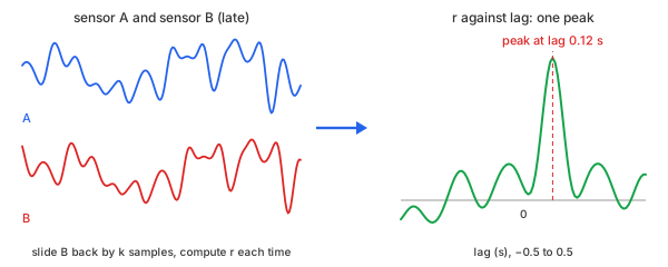
Fig 1. Slide one signal along the other; the best match is the delay
The measure of "how closely the two match" is the familiar correlation coefficient, Pearson's $r$, between $-1$ and $1$. Cross-correlation is Pearson's $r$ computed again at every time shift, or lag. A signal compared with itself is autocorrelation: its first peak after lag 0 is the period of whatever repeats in it.
Take an example: three columns sampled 100 times per second for 4 seconds—400 rows (Table 1). The example has two jobs, one for each kind of correlation.
- For cross-correlation, a delay to find. Column $y_1$ is sensor A, a smooth random motion with a little noise. Column $y_2$ is sensor B: the same motion arriving 0.12 s later, with more noise of its own.
- For autocorrelation, a repetition to find. Column $y_3$ is a separate signal: a 1.3 Hz sine of amplitude 1 with random noise added (standard deviation 0.5)—the kind of record a vibration sensor gives on a machine turning 78 times a minute. In the bold row, for example, the sine is 0.8306 and the noise −0.0659, so $y_3 = 0.7647$.
| t (s) | y1 (sensor A) | y2 (sensor B) | y3 (periodic) |
|---|---|---|---|
| 0.00 | 0.7079 | 1.4179 | −0.2737 |
| 0.01 | 0.8864 | 2.0423 | −0.2985 |
| 0.02 | 0.8830 | 1.3474 | 0.0156 |
| 0.12 | −0.2326 | 0.9614 | 0.7647 |
| 0.13 | −0.2499 | 0.9084 | 0.7429 |
| 0.50 | −0.2468 | 0.9433 | −0.6234 |
| 1.00 | −1.2693 | −0.0977 | 1.1489 |
| 2.00 | −0.4545 | 0.8526 | −1.0245 |
| 3.99 | −0.0052 | −0.7951 | 1.3739 |
Table 1. The example: 9 of its 400 rows
The bold row is 12 samples in: whatever sensor A recorded in the first row, sensor B records from here on.
Chart 1, for cross-correlation: the two sensors over the first 2 s. Sensor B follows the same ups and downs as sensor A, slightly later; the question is exactly how much later.
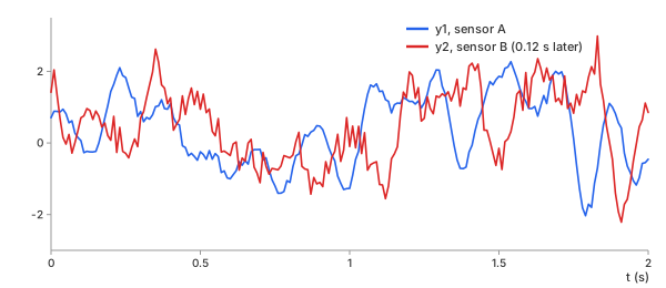
Chart 1. Cross-correlation's data: sensor A and sensor B, B later
Chart 2, for autocorrelation: $y_3$ over the whole 4 s, with the clean 1.3 Hz sine it was built from. The noise hides the sine sample by sample; the question is how often the record repeats.
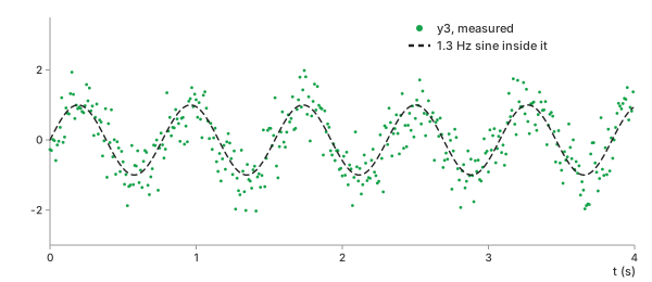
Chart 2. Autocorrelation's data: a noisy 1.3 Hz oscillation
The task: read the 0.12 s delay from $y_1$ and $y_2$, and the 1.3 Hz period from $y_3$, using only the data.
Methods
Four steps, each built on the one before: one number for two signals, that number at every lag, the same for one signal against itself, and a faster way to compute it.
Pearson's r
In plain words. Subtract each signal's mean, multiply the two sample by sample, and add up the products. Divide by what the sum would be if the two signals were identical. The result is 1 for a perfect match, 0 for no linear relation, and −1 for a mirror image.
Basic idea. Pearson's correlation coefficient for $N$ pairs $(x_n, y_n)$, with means $\bar{x}$, $\bar{y}$ and standard deviations $\sigma_x$, $\sigma_y$ (Math 1):
Math 1.
Example. For $y_1$ and $y_2$ as recorded, with $x = y_1$ and $y = y_2$. First the means and the standard deviations of all 400 values (Math 2):
Math 2.
Then, row by row, subtract each mean and multiply the two differences. The sum of the 400 products is the numerator of Math 1 (Table 2).
| row n | $x_n$ | $x_n - \bar{x}$ | $y_n$ | $y_n - \bar{y}$ | product |
|---|---|---|---|---|---|
| 0 | 0.7079 | 0.6266 | 1.4179 | 1.2786 | 0.8011 |
| 1 | 0.8864 | 0.8051 | 2.0423 | 1.9030 | 1.5321 |
| 2 | 0.8830 | 0.8017 | 1.3474 | 1.2081 | 0.9685 |
| … | … | … | … | … | … |
| 399 | −0.0052 | −0.0865 | −0.7951 | −0.9344 | 0.0808 |
| sum of all 400 products | 33.51 | ||||
Table 2. The numerator of Math 1, row by row
Divide by $N \sigma_x \sigma_y$ (Math 3):
Math 3.
Almost no relation—even though the two sensors recorded the same motion. The positive and negative products nearly cancel. The left panel of Chart 3 shows why: each point pairs sensor A's value with sensor B's value at the same moment, but B is 0.12 s behind, so the pairs do not belong together.
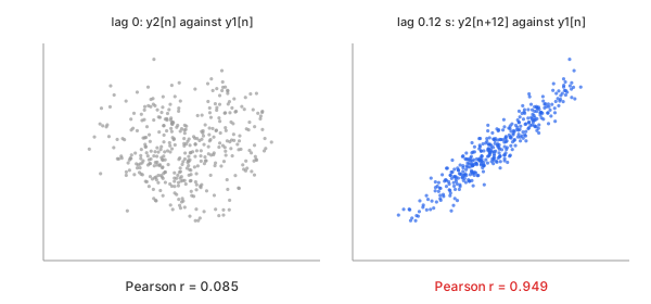
Chart 3. The same two signals, paired at the same moment and 0.12 s apart
The right panel pairs $x_n$ with $y_{n+12}$ instead: sample $n$ of sensor A with the sample of sensor B taken 0.12 s later. Only 388 such pairs exist, and Pearson's $r$ of those 388 pairs—with their own means $\bar{x}' = 0.0991$, $\bar{y}' = 0.1246$ and standard deviations $\sigma_x' = 0.9737$, $\sigma_y' = 1.0203$—is (Math 4):
Math 4.
Shifted into step, the two sensors agree almost perfectly. Cross-correlation, next, makes this shift systematic.
Important characteristics. Pearson's $r$ measures only a linear relation, and only between values paired as given.
Advantages
- One number, with a scale everyone reads the same way.
- Unaffected by the units, offset, or scale of either signal.
Disadvantages
- Blind to a time shift: two copies of one signal can score near 0.
- Sees only straight-line relations.
Cross-Correlation
In plain words. Repeat Pearson's $r$ with $y$ shifted by $k$ samples, for every $k$ in a range. Plot $r$ against $k$; the highest point is the delay.
Control parameters. maxLag (the largest $|k|$, given in
seconds on the calculators) sets how far the search goes; normalization
sets the divisor (see Biased or Unbiased).
Basic idea. At lag $k \ge 0$, sample $x_n$ is paired with $y_{n+k}$. Only $N - k$ pairs exist, but the divisor stays $N \sigma_x \sigma_y$ (Math 5). Negative lags pair $x_{n-k}$ with $y_n$ the same way.
Math 5.
At $k = 0$, Math 5 is Math 1: lag 0 of the cross-correlation is Pearson's $r$.
Example. At $k = 12$ samples, 0.12 s (Math 6):
Math 6.
The sum is the same as in Math 4, but the result, 0.9322, is a little lower than 0.9486: Math 5 keeps the means and standard deviations of the whole record and divides by $N = 400$, not by the 388 pairs (see Biased or Unbiased).
Chart 4 plots $r_{xy}(k)$ from −1 s to 1 s. One sharp peak stands out at 0.12 s; everywhere more than 0.05 s away from it, $r$ stays below 0.30.
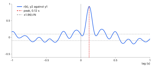
Chart 4. Cross-correlation of $y_2$ against $y_1$
Important characteristics. The peak gives the delay in samples; multiplied by the sampling interval, in seconds. The height of the peak says how alike the two signals are once aligned.
Advantages
- Finds a delay without any model of the signal itself.
- Works under heavy noise: every sample in the overlap votes.
Disadvantages
- Needs evenly spaced samples, so that a lag is one fixed time.
- The delay comes in whole samples unless the peak is refined (see Between Two Samples).
Autocorrelation
In plain words. Cross-correlate a signal with itself. At lag 0 it matches perfectly ($r = 1$); one period later it matches again.
Control parameters. The same maxLag and
normalization; it must reach past one period.
Basic idea. Math 5 with $y = x$ (Math 7). It is symmetric, so only $k \ge 0$ is needed.
Math 7.
Example. For $y_3$ (Chart 5), $r$ falls from 1, dips below 0 at half a period, and rises to its first peak, 0.520, at 0.78 s—one period of a 1.28 Hz oscillation, close to the true 1.3 Hz.
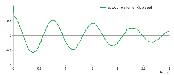
Chart 5. Autocorrelation of $y_3$
Important characteristics. Noise that is independent from sample to sample adds only to lag 0; at every other lag it averages out, which is why the period shows through.
Advantages
- Reads a period directly in seconds, without choosing frequency bins.
- Separates repeating structure from random noise.
Disadvantages
- The peaks shrink with lag (biased normalization), so later peaks are harder to read.
- Several periods at once overlap into one curve that is harder to read than a spectrum.
FFT-Based Correlation
In plain words. Split both records into sine waves, compare them one frequency at a time, and add the comparisons back together. The result is the same curve as Math 5, reached by a different route.
The core idea: the two sensors in the frequency domain. The Fourier transform describes each record as a sum of sine waves, one for each frequency, with an amplitude (how strong it is) and a phase (where its peaks fall in time). Chart 6 shows sensors A and B in this form.
- Amplitude: the same. A delay does not make any sine wave stronger or weaker, so the two amplitude curves lie almost on top of each other (left): on average, 0.208 and 0.205 between 0.5 Hz and 8 Hz. The small difference comes from B's noise.
- Phase: B falls behind A, increasingly at higher frequencies. On its own, each phase wanders with the shape of the random motion, so the same straight trend (the choice of time origin) is removed from both lines (right). The two lines then start together, and B drops below A by a gap that widens with frequency: 79° at 2 Hz, 192° at 4 Hz, and 268° at 6 Hz. At 0.977 Hz, for example, A's sine is at −123.2° and B's at −170.5°.
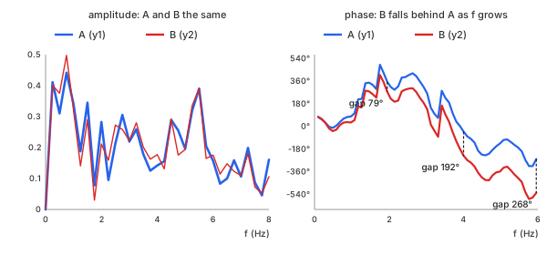
Chart 6. Sensors A and B in the frequency domain: the same amplitude, a phase gap that grows with frequency
The difference is a straight line. Subtract B's phase from A's at each frequency—at 0.977 Hz, $-123.2^\circ - (-170.5^\circ) = 47.3^\circ$—and the wandering shared by both lines cancels out, leaving only the gap (Chart 7). Delaying a sine wave of frequency $f$ by 0.12 s shifts its phase by $360^\circ \times f \times 0.12$ s: 43.2° at 1 Hz and 86.4° at 2 Hz. The phase lag of B behind A therefore grows linearly with frequency. A line fitted through the measured lags rises 43.5° per Hz, giving $43.5^\circ / 360^\circ = 0.1207$ s: the delay, read entirely in the frequency domain.
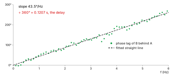
Chart 7. A's phase minus B's: a straight line whose slope is the delay
The FFT method does not fit this line. Instead, it multiplies the two transforms and transforms the result back: adding all the sine waves together with B's phase lags undone produces a curve that is large only where all the sine waves line up at once—the same single peak at 0.12 s as in Chart 4.
Basic idea. With $X$ and $Y$ the discrete Fourier transforms of the mean-removed signals, each zero-padded to a length $M \ge 2N - 1$ so that nothing wraps around (Math 8):
Math 8.
Each product $\overline{X} \cdot Y$ holds, for one frequency, how strong that sine is in both records and how far B's copy lags A's. The inverse transform (IDFT) performs the third step.
Example. The phases of $y_1$ and $y_2$ at five frequencies, B's lag behind A as read from $\overline{X} \cdot Y$, and the straight line of a 0.12 s delay (Table 3):
| frequency | phase of A | phase of B | lag, A − B | $360^\circ \times f \times 0.12$ s |
|---|---|---|---|---|
| 0.977 Hz | −123.2° | −170.5° | 47.3° | 42.2° |
| 1.953 Hz | −49.5° | −128.6° | 79.1° | 84.4° |
| 3.027 Hz | −41.0° | −165.8° | 124.8° | 130.8° |
| 4.004 Hz | 175.3° | −16.8° | 192.0° | 173.0° |
| 5.957 Hz | −87.1° | 4.7° | 268.2° | 257.3° |
Table 3. The phase lag of sensor B behind sensor A, by frequency
A phase is only known up to whole turns, so the lag is counted from 0° to 360°: at 5.957 Hz, $-87.1^\circ - 4.7^\circ = -91.8^\circ$, one turn short of $268.2^\circ$. The noise scatters each lag by a few degrees, but together they follow the line: a straight line fitted through all of them up to 6 Hz has the slope of a 0.1207 s delay. The frequencies are not round because the transform's bins are $f_s / M = 100 / 1024$ Hz apart. Over all 799 lags, the FFT method and the direct sums of Math 5 differ by at most $2.2 \times 10^{-16}$—rounding only.
Important characteristics. The same answer, at a lower cost: for all 799 lags of the example, the direct sums take 160,000 multiplications, and three transforms of length 1,024 take about 31,744 operations. The gap grows with the record: the direct sums grow as $N^2$, the FFT as $M \log_2 M$. For autocorrelation, $\overline{X} \cdot X = |X|^2$ is the power spectrum: the autocorrelation and the power spectrum are a Fourier pair (the Wiener–Khinchin theorem).
Advantages
- Fast for long records and many lags.
- Exactly the same result, when the zero-padding is long enough.
Disadvantages
- Without enough zero-padding, the end of the record wraps onto the start and corrupts every lag.
- No saving when only a few small lags are needed.
Which One Should You Choose?
| question | use | in the example |
|---|---|---|
| do two values move together, paired as recorded? | Pearson's $r$ | 0.0855 |
| how much later is one signal? | cross-correlation, peak lag | 0.12 s (r 0.932) |
| does one signal repeat, and how often? | autocorrelation, first peak | 0.78 s (1.28 Hz) |
| long record, all lags | FFT-based | same numbers, $2.2 \times 10^{-16}$ |
Table 4. What each method answers
The basic calculator computes cross- and autocorrelation in your browser, by direct sums. The advanced calculator adds the FFT method, any number of columns, a choice of reference column, and sub-sample peaks, computed on the server.
Key Ideas
The sums are simple. Reading them correctly takes six ideas.
The Sign of the Lag: Which Signal Is Late?
Lag $k$ in Math 5 pairs $x_n$ with $y_{n+k}$. A peak at a positive lag means $y$ is late: what $x$ does at sample $n$, $y$ does at sample $n + k$. A peak at a negative lag means $y$ is early.
Software does not agree on this convention. numpy.correlate(a, v) and
scipy.signal.correlate(in1, in2) both pair in1[n + k] with
in2[n], so the order of the arguments flips the sign. Both calculators here
use Math 5, with the reference column as $x$.
Biased or Unbiased: Fewer Pairs at Large Lags
At lag $k$, only $N - k$ pairs exist. The biased estimate (Math 5) still divides by $N$, so it shrinks toward 0 as the lag grows. The unbiased estimate divides by the number of pairs instead (Math 9).
Math 9.
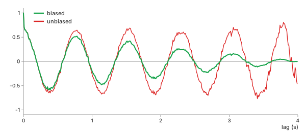
Chart 8. Biased and unbiased autocorrelation of $y_3$, every lag
| lag | pairs | biased | unbiased |
|---|---|---|---|
| 1.00 s | 300 | −0.195 | −0.260 |
| 2.00 s | 200 | −0.272 | −0.545 |
| 3.00 s | 100 | 0.149 | 0.595 |
| 3.80 s | 20 | 0.039 | 0.783 |
| 3.95 s | 5 | −0.004 | −0.338 |
Table 5. The same lags, biased and unbiased
The unbiased estimate keeps the size of the oscillation, but at 3.95 s it rests on 5 pairs and swings from 0.78 to −0.34 within 0.15 s. The biased estimate is smaller and steadier. Use biased by default, unbiased only for lags well under half the record, and never trust either beyond about a quarter of it.
Significance: The ±1.96/√N Band
Two unrelated white-noise records still give nonzero $r$ at every lag. For $N$ samples, about 95% of those values fall inside $\pm 1.96 / \sqrt{N}$; here $\pm 1.96 / \sqrt{400} = \pm 0.098$ (the dashed lines in Chart 4).
A peak far outside the band, like 0.932, is real. But the band assumes samples that are independent of their neighbors. Smooth signals are not: in Chart 4, $r$ crosses the band many times away from the peak and reaches 0.198 beyond 0.5 s. For smooth data, judge a peak by how far it stands above its neighbors, not by the band alone.
A Period in a Short Record: Autocorrelation Against the FFT
A Fourier transform of a 4 s record has bins $1 / 4 = 0.25$ Hz apart: 1.00, 1.25, 1.50 Hz, and so on. A 1.3 Hz tone falls between two of them, and the spectrum reports 1.25 Hz (Chart 9).
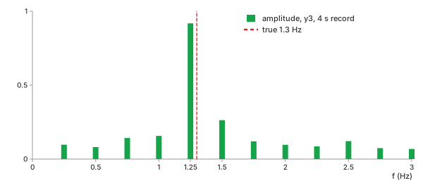
Chart 9. Spectrum of $y_3$: the tone falls between bins
| method | reads | error against 1.3 Hz |
|---|---|---|
| FFT, highest bin | 1.25 Hz | −3.8% |
| autocorrelation, first peak (refined) | 0.7772 s = 1.2866 Hz | −1.0% |
Table 6. The period of $y_3$ from a 4 s record
The autocorrelation measures time, not frequency, so it has no bins to fall between. Its own resolution is one sample, 0.01 s, and a parabola through the top of the peak refines it further (see Between Two Samples).
Traps: A Trend, and a Peak That Repeats
A trend correlates with itself at every lag. Adding a slow rise of $0.6\,t$ to $y_3$ lifts the whole autocorrelation: the dip at half a period goes from −0.554 to −0.031 and nearly disappears (Chart 10). Detrend first.
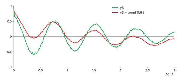
Chart 10. A trend fills in the autocorrelation's dips
A periodic signal matches itself every period, so its cross-correlation has a peak every period, and the tallest one is not always the true delay. A delay can only be read uniquely when it is shorter than half the period—or when the signal, like sensor A here, does not repeat. Filter out a strong periodic component before looking for a delay.
Between Two Samples: The Parabolic Peak
The peak lag is a whole number of samples, 0.01 s apart here. Near its top, a correlation peak is close to a parabola, so a parabola through the highest value $r_0$ and its two neighbors $r_-$ and $r_+$ places the true top between samples (Math 10).
Math 10.
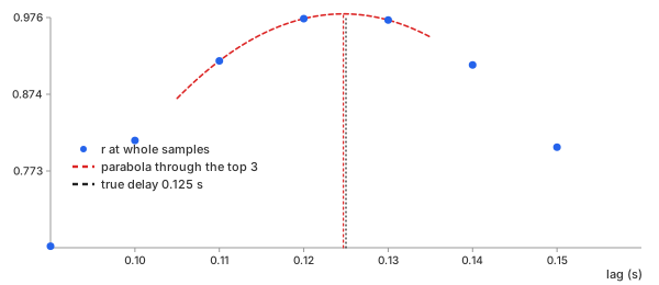
Chart 11. A delay of 12.5 samples, read as 12 samples and refined to 12.47
Delay sensor A's motion by 0.125 s—12.5 samples. The highest whole-sample value is at 12 samples (0.12 s); the parabola puts the peak at 12.469 samples, 0.1247 s. On the example itself, with noise, the refinement gives 0.1207 s for the true 0.12 s.
Shift, correlate, and read the peak—after removing the trend.
REFs
NumPy numpy.correlate SciPy scipy.signal.correlate SciPy scipy.signal.correlation_lags Wikipedia, Cross-correlation Wikipedia, Autocorrelation Wikipedia, Pearson correlation coefficient Wikipedia, Wiener–Khinchin theorem Fourier Transform (DFT, FFT): What Frequencies Are in My Data? Digital Filters: How to Keep Only the Frequencies You Want Detrending & Baseline Correction: How to Remove Drift from Measured Data