Correlation: Do Your Columns Move Together, and How Strongly?

An introduction to correlation: covariance and Pearson r, Spearman ρ and Kendall τ, the correlation matrix and heatmap, outliers, curves with r ≈ 0, and why correlation is not causation.

Contents

What Is Correlation? Do My Columns Move Together?
Covariance, Then Correlation
Methods
Which One Should You Choose?
Key Ideas
Example: Parameter Correlation in Curve Fitting
REFs

What Is Correlation? Do My Columns Move Together?

A sheet has several measured columns: two sensors read side by side, a temperature and a pressure, the price of two products week by week. The first question is usually the same: which of these columns move together, and how strongly?

Correlation answers with one number per pair, from −1 to 1: the correlation coefficient. Near 1, the two columns rise together along a straight line. Near −1, one falls as the other rises. Near 0, no straight line describes them. Fig 1 shows the three cases on three columns of the example introduced below: $y_1$, $y_2$ and $y_3$ against $x$.

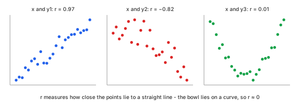
Three scatter plots against x: left, blue points rising along a line, r = 0.97; middle, red points falling with more scatter, r = −0.82; right, green points along a U-shaped bowl, r = 0.01

Fig 1. Three columns of the example (Chart 1) against $x$: $y_1$ rises, $y_2$ falls, and $y_3$ is a bowl that a straight line cannot describe

This distinguishes correlation from two related tools. Curve fitting gives an equation and predicts $y$; a correlation coefficient gives no equation, only how tight the straight-line relation is. Cross-correlation shifts one record against another in time and computes $r$ at every shift; correlation compares the columns row by row, with no shift.

Take an example: four columns measured at $x$ = 1, 1.5, 2, … 13—25 rows, all four drawn in Chart 1. Each one shows a different case; the first three are the panels of Fig 1.

$y_1$, rising. Made as $2 + 0.8\,x$ plus noise with a standard deviation of 1.0.
$y_2$, falling. Made as $12 - 0.6\,x$ plus noise with a standard deviation of 1.5: a weaker trend under more scatter.
$y_3$, a bowl. Made as $0.25\,(x - 7)^2$ plus noise with a standard deviation of 0.6: fully decided by $x$, but not along a line.
$y_4$, a decay. Made as $10\,e^{-0.3\,x}$ plus noise with a standard deviation of 0.2: always falling, but along a curve.

Chart 1 shows the four columns as measured, the same values every later chart of them uses: $y_1$ runs from 2 to 13.6, $y_2$ from 3 to 11.4, $y_3$ from −0.8 to 9 and $y_4$ from 0.2 to 7.5.

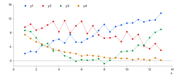
The four columns against x as measured: blue y1 rising from 2 to 13.6, red y2 falling from about 10 to 3 with large jumps, green y3 falling from 8.7 to near 0 and rising back to 9 in a U, orange y4 falling fast from 7.5 then flattening near 0.2

Chart 1. The four columns of the example against $x$, as measured

Covariance, Then Correlation

Start with each point's distance from the means. When $x$ is above its mean $\bar{x}$ and $y$ is above its mean $\bar{y}$, the product $(x - \bar{x})(y - \bar{y})$ is positive; it is also positive when both are below. When one is above and the other below, the product is negative. The average of these products is the covariance (Math 1); Chart 2 draws these products for one pair of the example:

$$\operatorname{cov}(x, y) = \frac{1}{N - 1}\sum_{i=1}^{N} (x_i - \bar{x})(y_i - \bar{y}) = \frac{(x_1 - \bar{x})(y_1 - \bar{y}) + \dots + (x_N - \bar{x})(y_N - \bar{y})}{N - 1}$$

$$\begin{aligned} \operatorname{cov}(x, y) &= \frac{1}{N - 1}\sum_{i=1}^{N} (x_i - \bar{x})(y_i - \bar{y}) \\ &= \frac{1}{N - 1}\big[(x_1 - \bar{x})(y_1 - \bar{y}) \\ &\qquad + \dots + (x_N - \bar{x})(y_N - \bar{y})\big] \end{aligned}$$

Math 1.

Chart 2 shows the products of Math 1 for $x$ and $y_2$, the falling column of Chart 1. The means $\bar{x} = 7$ and $\bar{y} = 7.857$ split the plane into four quadrants. 22 of the 25 points sit in the two quadrants where the product is negative, so the covariance is negative: $y_2$ falls as $x$ rises.

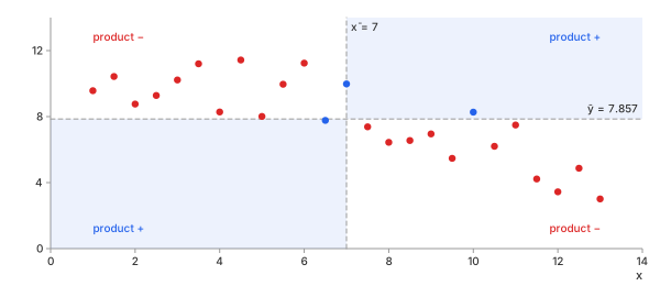
x against y2 with dashed lines at the means x̄ = 7 and ȳ = 7.857; 22 red points in the top-left and bottom-right quadrants where the product is negative, 3 blue points near the centre where it is positive

Chart 2. $x$ against $y_2$ of Chart 1: the products $(x - \bar{x})(y - \bar{y})$ of Math 1, red where negative, blue where positive

The covariance has one problem: it carries the units of both columns. For the $x$ and $y_2$ of Chart 2 it is −7.2871. Write $y_2$ in centimetres instead of metres—every value times 100—and the covariance becomes −728.71, though nothing about the relation changed. Dividing by both standard deviations removes the units and gives a number between −1 and 1: the correlation coefficient (Math 2, next). For $y_2$ it is −0.8165 in either unit.

Methods

Three coefficients are in common use. Pearson's works on the values, Spearman's and Kendall's on their order. All three read the same way: 1 a perfect rise, −1 a perfect fall, 0 none.

Pearson r

In plain words. The Pearson correlation coefficient ($r$) is the covariance with the units divided out. It measures how close the points lie to a straight line—any straight line, steep or shallow.

Control parameters. None: $r$ is fixed by the data. The advanced calculator's confidence level (level) sets only the width of the interval around $r$ (Math 8).

Basic idea. Pearson's product-moment correlation. With the standard deviations $s_x$ and $s_y$ (Math 2):

$$r = \frac{\operatorname{cov}(x, y)}{s_x\,s_y} = \frac{\sum_{i=1}^{N} (x_i - \bar{x})(y_i - \bar{y})}{\sqrt{\sum_{i=1}^{N} (x_i - \bar{x})^2}\,\sqrt{\sum_{i=1}^{N} (y_i - \bar{y})^2}} = \frac{(x_1 - \bar{x})(y_1 - \bar{y}) + \dots + (x_N - \bar{x})(y_N - \bar{y})}{\sqrt{(x_1 - \bar{x})^2 + \dots}\,\sqrt{(y_1 - \bar{y})^2 + \dots}}$$

$$\begin{aligned} r &= \frac{\operatorname{cov}(x, y)}{s_x\,s_y} \\ &= \frac{\sum_{i=1}^{N} (x_i - \bar{x})(y_i - \bar{y})}{\sqrt{\sum_{i=1}^{N} (x_i - \bar{x})^2}\,\sqrt{\sum_{i=1}^{N} (y_i - \bar{y})^2}} \\ &= \frac{(x_1 - \bar{x})(y_1 - \bar{y}) + \dots}{\sqrt{(x_1 - \bar{x})^2 + \dots}\,\sqrt{(y_1 - \bar{y})^2 + \dots}} \end{aligned}$$

Math 2.

Why divide by both spreads: the covariance grows with the size of either column; dividing by $s_x\,s_y$ leaves only how well the two move together. It standardises each column—its mean subtracted, the result divided by its standard deviation, so every column centres on 0 with a spread of 1—and $r$ is the sum of the products of the standardised values, divided by $N - 1$. The calculator's first chart shows the columns of Chart 1 standardised this way.
Range: always from −1 to 1; ±1 only when every point lies on one straight line.
Symmetric: $r(x, y) = r(y, x)$; neither column is the "input".
If a column is constant: its spread is 0, and $r$ is not defined.

Example. Take the first five rows of $x$ and $y_1$ from Chart 1 (Table 1); Chart 3 draws them. The $x$ values add up to 10 and the $y_1$ values to 15.71, so $\bar{x} = 2$ and $\bar{y} = 3.142$.

$x$	$y_1$	$x - \bar{x}$	$y_1 - \bar{y}$	$(x - \bar{x})(y_1 - \bar{y})$	$(x - \bar{x})^2$	$(y_1 - \bar{y})^2$
1	2.07	−1.0	−1.072	1.0720	1.00	1.1492
1.5	2.66	−0.5	−0.482	0.2410	0.25	0.2323
2	2.54	0.0	−0.602	0.0000	0.00	0.3624
2.5	4.44	0.5	1.298	0.6490	0.25	1.6848
3	4.00	1.0	0.858	0.8580	1.00	0.7362
sum				2.8200	2.50	4.1649

Table 1. The first five rows of $x$ and $y_1$, the three sums of Math 2

Then the three sums of Table 1 go into Math 2 (Math 3):

$$r = \frac{2.8200}{\sqrt{2.50 \times 4.1649}} = 0.8739$$

Math 3.

Chart 3 draws the same five rows around the means of Table 1. Each product of Math 2 is a rectangle from the mean cross to the point, blue when positive. Four are positive and the third row sits on $\bar{x}$, so its product is 0: the sum 2.82, and with it $r$, is positive.

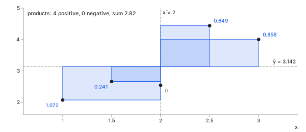
The five rows of Table 1 as points with dashed mean lines at x̄ = 2 and ȳ = 3.142; from the crossing, a blue rectangle to each point labelled with its product: 1.072, 0.241, 0.649, 0.858, and 0 for the point on the x̄ line; sum 2.82

Chart 3. The five rows of Table 1: each product $(x - \bar{x})(y_1 - \bar{y})$ of Math 2 as a rectangle from the means

Over all 25 rows of Chart 1, the same formula gives $r = 0.9664$.

Important characteristics. One closed-form step; it uses every value as it is, so it sees how far each point is from the line.

Advantages

The standard: every tool reports it, and it links straight to a fitted line.
Uses the full values, so it has the most power on clean, roughly straight data.

Disadvantages

Straight lines only: a steady curve scores less than 1 (Chart 5), a bowl about 0 (Fig 1).
Squared distances: one far point can move it a long way (Chart 9).

Spearman ρ

In plain words. The Spearman rank correlation ($\rho$) replaces each value by its rank—1 for the smallest, 2 for the next—and takes Pearson's $r$ of the ranks. It asks whether $y$ always rises (or always falls) with $x$, along any curve, not only a straight line.

Control parameters. None, as for Pearson.

Basic idea. Spearman's rank correlation. With $d_i$ the difference between the two ranks of row $i$, and no tied values (Math 4):

$$\rho = 1 - \frac{6\sum_{i=1}^{N} d_i^2}{N\,(N^2 - 1)}, \qquad \sum_{i=1}^{N} d_i^2 = d_1^2 + d_2^2 + \dots + d_N^2$$

$$\begin{aligned} \rho &= 1 - \frac{6\sum_{i=1}^{N} d_i^2}{N\,(N^2 - 1)} \\ \sum_{i=1}^{N} d_i^2 &= d_1^2 + d_2^2 + \dots + d_N^2 \end{aligned}$$

Math 4.

Why ranks: a rank keeps only the order, so any curve that always rises becomes a straight line of ranks.
Ties: equal values share the average of their ranks; Math 4 is then only close, and Pearson's $r$ of the ranks is exact.
Reading it: 1 means $y$ never falls when $x$ rises.

Example. The same five rows as Table 1, now as ranks (Table 2), drawn in Chart 4. $y_1$ swaps order twice: 2.66 before 2.54, and 4.44 before 4.00.

$x$	$y_1$	rank $x$	rank $y_1$	$d$	$d^2$
1	2.07	1	1	0	0
1.5	2.66	2	3	−1	1
2	2.54	3	2	1	1
2.5	4.44	4	5	−1	1
3	4.00	5	4	1	1
sum					4

Table 2. The first five rows of $x$ and $y_1$, as ranks

The four $d^2$ of Table 2 go into Math 4 (Math 5):

$$\rho = 1 - \frac{6 \times 4}{5 \times (25 - 1)} = 1 - \frac{24}{120} = 0.8000$$

$$\begin{aligned} \rho &= 1 - \frac{6 \times 4}{5 \times (25 - 1)} \\ &= 1 - \frac{24}{120} = 0.8000 \end{aligned}$$

Math 5.

Chart 4 shows the same ranks: the five rows as values, then as ranks. Each swap moves two points off the dashed line of equal ranks, one by +1 and one by −1.

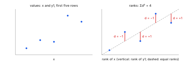
Left, the five rows of Table 2 as values of x and y1. Right, the same rows as ranks with a dashed line of equal ranks; four points sit off it, each joined to it by a red line labelled d = −1 or d = +1; Σd² = 4

Chart 4. The five rows of Table 2: values, then ranks; each $d$ of Math 4 is the distance to the dashed line of equal ranks

Chart 5 shows where ranks matter: $y_4$ of Chart 1 falls at every step but along a curve. Pearson's $r$ is −0.8984; the ranks lie almost on a line, and $\rho = -0.9715$.

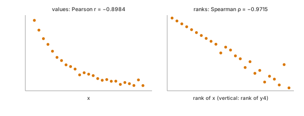
Left, x against y4 as values: orange points falling along a curve, Pearson r = −0.8984. Right, the same rows as ranks: the points fall almost along a straight line, Spearman ρ = −0.9715

Chart 5. $x$ against $y_4$ of Chart 1: the values follow a curve, the ranks a line

Important characteristics. Sorting first, then Pearson on the ranks: the size of a step no longer counts, only its direction.

Advantages

Catches any steady rise or fall, curved or straight.
An extreme value is only the top or bottom rank, however far it is (Chart 9).

Disadvantages

Throws away the sizes: a rise of 0.01 counts as much as a rise of 10.
Still blind to a bowl: $y_3$ falls and rises (Fig 1, right), and $\rho = 0.0054$.

Kendall τ

In plain words. The Kendall rank correlation ($\tau$) looks at every pair of rows. A pair is concordant when $x$ and $y$ move the same way between the two rows, discordant when they move opposite ways. $\tau$ is the share of concordant pairs minus the share of discordant ones.

Control parameters. None, as for Pearson.

Basic idea. Kendall's rank correlation. With $C$ concordant and $D$ discordant pairs among the $N(N - 1)/2$ pairs, and no ties (Math 6):

$$\tau = \frac{C - D}{N\,(N - 1)/2}$$

Math 6.

Why pairs: a pair either agrees or disagrees, so $\tau$ reads directly as a probability: $(1 + \tau)/2$ of the pairs agree.
Ties: a tied pair is neither; the advanced calculator uses $\tau_b$, which corrects the denominator for ties.
Size: for the same data, $|\tau|$ is usually smaller than $|\rho|$—a different scale, not a weaker relation.

Example. The same five rows as Table 1 give 10 pairs (Table 3); Chart 6 joins each pair with a line.

rows	$\Delta x$	$\Delta y_1$	pair
1, 2	+0.5	+0.59	concordant
1, 3	+1	+0.47	concordant
1, 4	+1.5	+2.37	concordant
1, 5	+2	+1.93	concordant
2, 3	+0.5	−0.12	discordant
2, 4	+1	+1.78	concordant
2, 5	+1.5	+1.34	concordant
3, 4	+0.5	+1.90	concordant
3, 5	+1	+1.46	concordant
4, 5	+0.5	−0.44	discordant

Table 3. Every pair of the first five rows of $x$ and $y_1$

8 concordant and 2 discordant pairs go into Math 6 (Math 7):

$$\tau = \frac{8 - 2}{5 \times 4 / 2} = \frac{6}{10} = 0.6000$$

Math 7.

Chart 6 draws the pairs of Table 3. Its two red lines are the two swaps already seen in Table 2 and Chart 4.

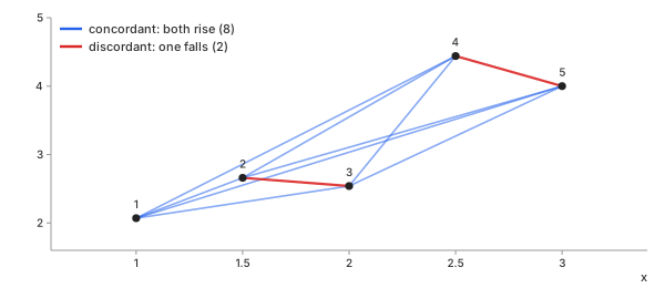
The five rows of Table 3 as numbered points; all ten pairs joined by lines: eight blue lines for concordant pairs that rise together, two red lines, rows 2-3 and 4-5, for discordant pairs where y1 falls

Chart 6. Every pair of the five rows of Table 3: blue concordant, red discordant

The same five rows give $r = 0.8739$ (Math 3), $\rho = 0.8000$ (Math 5) and $\tau = 0.6000$ (Math 7): three scales, one relation.

Important characteristics. Counts pairs, $N(N - 1)/2$ of them: 300 for 25 rows, about 50 million for 10,000.

Advantages

A plain meaning: the chance that two rows agree, minus the chance they disagree.
Like Spearman, an extreme value counts only as one more pair out of order (Chart 9); well behaved on small samples.

Disadvantages

Its numbers run smaller than $r$ and $\rho$, so values are not comparable across methods.
More work: every pair, not every row.

Which One Should You Choose?

Table 4 puts the three side by side for $x$ against each column of Chart 1, and Chart 7 draws it as bars.

column	Pearson $r$	Spearman $\rho$	Kendall $\tau$	shape
$y_1$	0.9664	0.9646	0.8667	rising line
$y_2$	−0.8165	−0.8138	−0.6200	falling line, more scatter
$y_3$	0.0055	0.0054	0.0133	bowl
$y_4$	−0.8984	−0.9715	−0.9133	falling curve

Table 4. The three coefficients for $x$ against each column

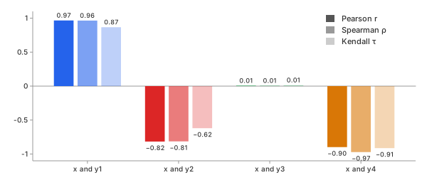
Grouped bars for x against y1, y2, y3, y4, three bars each for Pearson r, Spearman ρ and Kendall τ in the column's colour: tall positive for y1 (0.97, 0.96, 0.87), negative for y2 (−0.82, −0.81, −0.62), almost nothing for y3, negative for y4 with Spearman the longest (−0.90, −0.97, −0.91)

Chart 7. Table 4 as bars: $r$, $\rho$ and $\tau$ for $x$ against each column, in the column's colour from Chart 1

A straight-line relation, clean data: Pearson $r$. It agrees with the ranks on $y_1$ and $y_2$ and uses the most information.
A steady rise or fall along a curve: Spearman $\rho$. On $y_4$ it finds −0.9715 where Pearson finds −0.8984 (Chart 5).
Outliers, small samples, or many ties: Kendall $\tau$ or Spearman $\rho$.
A bowl or a wave: none of the three. Look at the scatter plot, and fit a curve instead.

When Pearson and Spearman disagree, the difference is itself the finding: the relation is curved, or a few points carry it.

Key Ideas

Look at the Scatter Plot First

A correlation coefficient compresses a whole cloud of points into one number, and very different clouds compress to the same one. Anscombe's quartet is four sets of 11 points built in 1973 to show this (Chart 8). All four have $r \approx 0.816$, the same means, and the same fitted line.

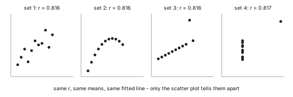
Anscombe's four data sets side by side, each with r = 0.816 or 0.817: a noisy rising cloud, a smooth arch, a perfect line with one high point, and a vertical stack with one far point to the right

Chart 8. Anscombe's quartet: four pictures, one $r$

Set 1 (Chart 8, first panel): what $r = 0.816$ is meant to describe—a noisy line.
Set 2: a smooth curve, where a line is the wrong model.
Set 3: a perfect line, pulled down by one point.
Set 4: no relation at all, created by one point.

The calculator therefore shows a scatter plot beside every number.

A Perfect Curve Can Score r ≈ 0

$y_3$ is decided by $x$ almost exactly: the bowl $0.25\,(x - 7)^2$ plus a little noise. Yet $r = 0.0055$ (Fig 1, right). On the left half, $y_3$ falls as $x$ rises; on the right half, it rises. The negative products of one half cancel the positive products of the other in Math 1—the quadrant picture of Chart 2, with points in all four quadrants.

Ranks do not help: $\rho = 0.0054$ and $\tau = 0.0133$ (Chart 7, $y_3$). All three coefficients ask about one direction, and a bowl has two. $r \approx 0$ means no straight-line relation, never "no relation".

Outliers: One Point Moves Pearson r

Replace one reading of $y_1$ of Chart 1, at $x = 7$, from 7.04 by 30—a typing slip or a sensor spike (Chart 9). Table 5 then pushes that reading further and further up.

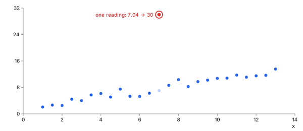
x against y1 with one reading at x = 7 moved from 7.04 up to 30, circled in red, far above the rising line of the other points

Chart 9. $x$ against $y_1$ of Chart 1, one reading replaced by 30

reading at $x = 7$	Pearson $r$	Spearman $\rho$	Kendall $\tau$
7.04 (original)	0.9664	0.9646	0.8667
16	0.8656	0.9077	0.7933
20	0.7777	0.9077	0.7933
30	0.5779	0.9077	0.7933
60	0.2927	0.9077	0.7933

Table 5. One reading of $y_1$ pushed further and further up

In Table 5, Pearson's $r$ keeps falling as the reading grows, because the distance is squared—the reading's product in Math 2 grows with it, as one huge rectangle would in Chart 3. Spearman and Kendall move once—the reading becomes the top rank—and then stop: 16, 30 or 60 is the same rank. When the two kinds disagree this much, find the point before trusting either number.

The Correlation Matrix and Its Heatmap

With $n$ columns there are $n(n - 1)/2$ pairs: 10 for the five columns of Chart 1, $x$ included. The correlation matrix holds them all, row $i$ and column $j$ the coefficient of columns $i$ and $j$. The diagonal is 1, and the matrix is symmetric. A heatmap colours each cell: blue for positive, red for negative, white near 0 (Chart 10).

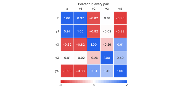
A five-by-five heatmap of Pearson r for x, y1, y2, y3, y4: deep blue 0.97 for x and y1, red −0.82 and −0.90 for x with y2 and y4, near-white 0.01 for x and y3, light blue 0.61 for y2 and y4 and 0.40 for y3 and y4

Chart 10. Pearson $r$ for every pair of the five columns of Chart 1

Chart 10 is read in seconds; its top row repeats the Pearson bars of Chart 7: $x$, $y_1$, $y_2$ and $y_4$ form one block of strong cells, and $y_3$ stands apart. Its pale cells against $x$ do not mean $y_3$ is unrelated—it is the bowl of Fig 1. In the calculator, a click on a cell shows that pair's scatter plot.

The Confidence Ellipse

For a cloud of points shaped like a normal distribution, an ellipse drawn from the two means and the covariance shows where most points sit. Its radius is set so it holds a chosen share, 95% here (Chart 11, on $y_1$ and $y_3$ of Chart 1). Strong correlation makes it narrow and tilted along the line; $r \approx 0$ makes it upright, with its axes along $x$ and $y$.

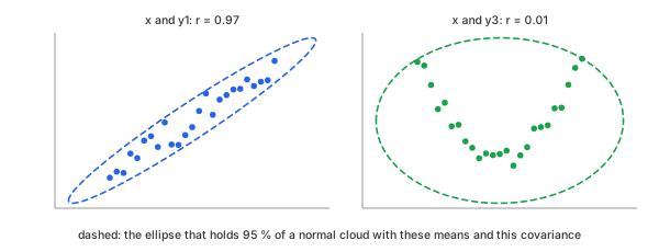
Left, x against y1 with a narrow dashed blue ellipse tilted along the rising points, r = 0.97. Right, x against y3 with a wide upright dashed green ellipse around the U-shaped points, r = 0.01

Chart 11. The 95% ellipse: narrow and tilted for $x$, $y_1$; wide and upright for $x$, $y_3$

In Chart 11 the ellipse also shows what a normal cloud would look like. On $x$, $y_3$ the points climb to its upper edge at both ends and leave the centre and the bottom empty—another sign that a bowl is not a cloud.

Correlation Is Not Causation

$y_1$ and $y_4$ have $r = -0.8794$ (Chart 10). Neither was made from the other: both were made from $x$, one rising and one falling. A third quantity that drives both columns is a confounder, and it creates a strong correlation without any link between the two.

Common cause: ice cream sales and sunburns rise together; summer drives both.
Reverse direction: $r$ is symmetric, so it cannot say which column drives which.
Chance: $y_3$ and $y_4$ give $r = 0.4002$ with $p = 0.047$, under the usual 0.05 line, though neither was made from the other.

A correlation is a reason to look for a mechanism, never the mechanism itself. See correlation does not imply causation.

How Sure Is r? p-Value and Confidence Interval

A coefficient from 25 rows is an estimate. To see how far chance alone moves it, take two columns of 25 random numbers with no relation at all, compute $r$, and repeat 2,000 times (Chart 12).

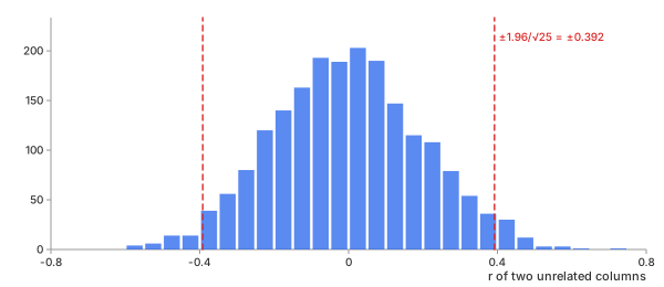
Histogram of r from 2,000 pairs of unrelated 25-row columns: a bell centred on 0, spread from about −0.6 to 0.7, with dashed red lines at ±0.392

Chart 12. $r$ of two unrelated columns of 25 rows, 2,000 times

Spread: the values of $r$ have a standard deviation of 0.2000, close to $1/\sqrt{N - 1} = 0.2041$.
Large by chance: 33% of the runs give $|r| > 0.2$, and the largest is 0.706.
The 5% line: 4.9% of the runs fall beyond $\pm 1.96/\sqrt{25} = \pm 0.392$.

So with 25 rows, a cell of the matrix in Chart 10 near ±0.2 or ±0.3 can be pure noise. Two numbers say how much:

p-value: the chance of an $|r|$ at least this large if the two columns were unrelated. For 25 rows, $p < 0.05$ needs $|r| > 0.3961$.
Confidence interval: the range of correlations consistent with the data. It comes from the Fisher transformation, which makes the spread of $r$ even (Math 8). Chart 13 draws the result.

$$z = \operatorname{artanh} r, \qquad z \pm \frac{1.96}{\sqrt{N - 3}}, \qquad \text{back through } r = \tanh z$$

$$\begin{aligned} z &= \operatorname{artanh} r \\ z &\pm \frac{1.96}{\sqrt{N - 3}} \\ r &= \tanh z \end{aligned}$$

Math 8.

Math 8 on two pairs of Chart 1 (Chart 13). For $x$ and $y_1$, $r = 0.9664$ with a 95% interval from 0.9243 to 0.9853: strong beyond doubt. For $x$ and $y_3$, $r = 0.0055$ with an interval from −0.3905 to 0.3998: the data cannot tell a moderate correlation from none—the interval spans the dashed lines at ±0.392 of Chart 12.

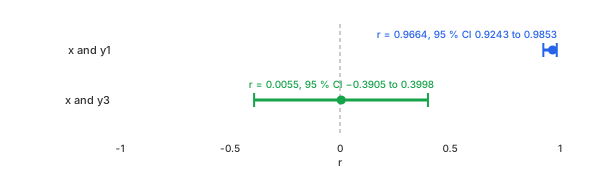
Two horizontal interval bars on an r axis from −1 to 1 with a dashed line at 0: x and y1, a short blue bar from 0.9243 to 0.9853 around r = 0.9664; x and y3, a long green bar from −0.3905 to 0.3998 around r = 0.0055

Chart 13. $r$ and its 95% interval from Math 8, for $x$ against $y_1$ and $y_3$ of Chart 1

Spearman's and Kendall's intervals use the same transformation, each with its own spread. The advanced calculator gives the p-value and interval for every pair.

Example: Parameter Correlation in Curve Fitting

Correlation also describes the result of a fit. The curve fitting blog fits $y = 1 + 2.2\,x - 0.16\,x^2$ plus noise on the same $x$. Make that data 25 times, each with new noise (standard deviation 0.4, random seed 7), and fit a cubic $c_0 + c_1 x + c_2 x^2 + c_3 x^3$ each time. The 25 sets of four coefficients are four columns, and their correlation matrix—the heatmap of Chart 10, now for coefficients—shows how they move together (Chart 14, left).

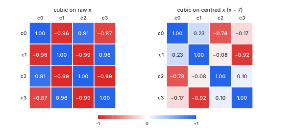
Two four-by-four heatmaps of the cubic's coefficients c0 to c3 over 25 fits. Left, on raw x: a strong checkerboard, −0.96, 0.91, −0.87, −0.99, 0.96, −0.99. Right, on x − 7: mostly pale, with −0.78 for c0 and c2 and −0.92 for c1 and c3

Chart 14. Correlation of the cubic's coefficients over 25 fits: raw $x$, then centred $x - 7$

Raw $x$ (Chart 14, left): a strong ± checkerboard, $|r|$ from 0.87 to 0.99. A little more $c_1$ is offset by a little less $c_0$ and $c_2$; the curve barely changes, so the data cannot pin each coefficient down. $c_0$ wanders with a standard deviation of 0.4845.
Centred, $x - 7$ (Chart 14, right): most cells pale. $c_0$ is now the value at the middle of the data, not at $x = 0$ far outside it, and its standard deviation falls to 0.1084.
What stays: $c_0$ with $c_2$ ($r = -0.7848$) and $c_1$ with $c_3$ ($r = -0.9222$). Even powers trade with even powers, odd with odd.

The second case is a decay $a\,e^{-b x} + c$ fitted to $10\,e^{-0.3 x}$ plus noise (standard deviation 0.2), again 25 times (Chart 15).

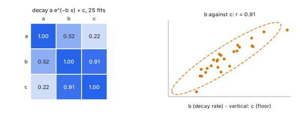
Left, a three-by-three heatmap of a, b, c over 25 decay fits: a with b 0.52, a with c 0.22, b with c 0.91. Right, b against c: 25 orange points rising along a narrow dashed ellipse, r = 0.91

Chart 15. The decay's three coefficients over 25 fits, and $b$ against $c$

$b$ and $c$ have $r = 0.9137$, with a 95% interval from 0.8116 to 0.9616 (Math 8), drawn with its ellipse in Chart 15, right. A faster decay (larger $b$) drops the curve sooner, and a higher floor $c$ lifts the tail back to the data: the two trade off. A strong cell between two coefficients means the data constrain their combination, not each one alone. Centring $x$, more data at the tail, or a fixed floor breaks the trade.

A correlation coefficient summarises a straight-line relation in one number. Look at the scatter plot, check how sure the number is, and never read it as a cause.

REFs

NIST/SEMATECH e-Handbook, Scatter Plot NIST/SEMATECH e-Handbook, Mean Vector and Covariance Matrix NumPy numpy.corrcoef SciPy scipy.stats.pearsonr SciPy scipy.stats.spearmanr SciPy scipy.stats.kendalltau Wikipedia, Correlation Wikipedia, Covariance Wikipedia, Pearson correlation coefficient Wikipedia, Spearman's rank correlation coefficient Wikipedia, Kendall rank correlation coefficient Wikipedia, Anscombe's quartet Wikipedia, Fisher transformation Wikipedia, Correlation does not imply causation Curve Fitting: Which Equation Fits My Data, and How Well? Cross-Correlation & Autocorrelation: How Far Apart Are Two Signals?