How to find and measure peaks using local maxima, prominence, derivative and wavelet methods, FWHM, and fits of overlapping Gaussian, Lorentzian and Voigt peaks.
Contents
What Is Peak Finding? Which Bumps Are Real Peaks?
A Raman or X-ray spectrum, a chromatogram, or an ECG trace is a curve with bumps, and those bumps carry the information. Each may mark a compound, a crystal plane, or a heartbeat. The questions are the same: which bumps are real peaks, where exactly is each one, and how tall and wide is it?
Peak finding answers in two stages. The first stage finds the peaks: it decides which bumps count and gives a position and a rough height for each. The second stage measures them: the width, the shape, the area, and a refined position and height, even where two peaks overlap.
Consider two example data columns, $y_1$ and $y_2$, each measured at 401 points from $x$ = 0 to 100 in steps of 0.25. Chart 1 shows the resulting data.
- $y_1$, three separate peaks. Constructed from a Gaussian peak of amplitude 1.0 at $x$ = 20 and width 4, a Lorentzian peak of amplitude 0.7 at $x$ = 50 and width 6, and a Gaussian peak of amplitude 0.5 at $x$ = 78 and width 8. A constant offset of 0.1 and noise with a standard deviation of 0.02 are added. The width here is the full width at half maximum, defined in Math 5 below.
- $y_2$, two peaks that overlap. Constructed from two Gaussian peaks, with amplitudes 1.0 and 0.6 at $x$ = 46 and 54, respectively, and a width of 10 for each. The same offset is added, along with noise with a standard deviation of 0.01. The peaks are separated by less than one FWHM, so they merge into a single bump with a shoulder.
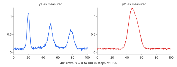
Chart 1. The two columns of the example against $x$, as measured
Every later chart of $y_1$ or $y_2$ shows these same values, on the same scale.
A Local Maximum First: Easy, and Not Enough
The simplest definition of a peak is a local maximum: a sample whose value is higher than those of both neighbouring samples (Math 1). A flat top, equal samples side by side, has its own rule; see Plateaus below.
Math 1.
Table 1 applies Math 1 to nine samples of $y_1$ around the first peak, from $x$ = 19 to 21. Only the sample at $x$ = 19.75 qualifies: its value, 1.0888, is higher than both neighbouring values, 1.0837 and 1.0875.
| $x$ | 19 | 19.25 | 19.5 | 19.75 | 20 | 20.25 | 20.5 | 20.75 | 21 |
|---|---|---|---|---|---|---|---|---|---|
| $y_1$ | 0.9234 | 0.9881 | 1.0837 | 1.0888 | 1.0875 | 1.0736 | 1.0732 | 0.9933 | 0.9229 |
| local max | no | no | no | yes | no | no | no | no | no |
Table 1. Math 1 on nine samples of $y_1$ from Chart 1
The rule takes only one line of code, but it is not sufficient for real data. Chart 2 marks every local maximum of $y_1$ from Chart 1: there are 116, and only 3 of them are peaks. The noise makes a small local maximum every few samples, on the baseline and on the flanks of the real peaks alike.
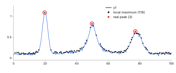
Chart 2. Every local maximum of $y_1$ (Math 1): 116 black dots, the 3 real peaks circled in red
The challenge in peak finding is deciding which of these maxima should count as peaks.
Methods: Find, Then Measure
The methods fall into two stages. Chart 3 illustrates both stages using $y_2$ from Chart 1. Stage 1 (left) detects one maximum at $x$ = 47 and measures its width directly from the data. Stage 2 (right) fits two peak functions (green dashed lines). Their sum (the red line) follows the data and reveals the second peak hidden in the shoulder.
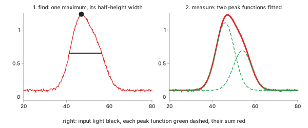
Chart 3. The two stages on $y_2$ of Chart 1: find (left), then measure (right)
- Stage 1, find: where the peaks are, and roughly how tall. Three methods: local maximum with filters, derivative zero-crossing, continuous wavelet transform.
- Stage 2, measure: how wide, what shape, what area, and the exact position and height. Two methods: half-prominence width and peak function fit.
Stage 1, Find: Position and Rough Height
Local Maximum and Filters
In plain words. Take every local maximum of Math 1, then keep only the ones that pass filters. The most important filter is prominence: how far a peak rises above the higher of the two surrounding bases that separate it from higher peaks. A noise maximum stands a few hundredths above its neighbours; a real peak stands far above its surroundings.
Control parameters. prominence (the minimum $P$ in
Math 2, expressed as a fraction of the data range; 0.1 by default), height
(the minimum allowed value of $y_i$; disabled by default), and distance (the
minimum separation between retained peaks, in samples; 1 by default). The advanced
calculator also provides width, plateau and
threshold filters.
Basic idea. Starting at a peak at sample $i$, move left and right until the signal rises above $y_i$ again, on the flank of a higher peak, or the end of the record is reached. No search window is specified here, so the search can extend across the entire record. The lowest point on each side is a base, $b_L$ and $b_R$. The higher of the two bases defines the reference level from which the peak's prominence is measured (Math 2):
Math 2.
- Why prominence: a height alone cannot tell a noise maximum on the flank of a tall peak from a small real peak; both may sit at the same height. Their prominences differ by an order of magnitude.
- Prominence on $y_1$: Chart 4 draws $P$ for every local maximum of $y_1$ from Chart 1. The three peaks have prominence values of 1.02, 0.74 and 0.55, while the largest noise maximum has a prominence of 0.069. A limit of 10 % of the range, 0.104, keeps exactly the three.
- Scale-free: when expressed as a fraction of the data range, the threshold is independent of the units—for example, whether the data are counts in the thousands or absorbance values in hundredths.
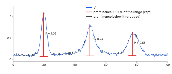
Chart 4. Prominence $P$ (Math 2) of every local maximum of $y_1$: red where $P \ge$ 10 % of the range, gray below
Advantages
- Exact: no smoothing, no model; positions are samples of the data.
- Interpretable: each filter is one number with a meaning in the data's own units.
- Fast: no iteration. A single pass identifies the local maxima; prominence is then calculated by searching outward from each candidate.
Disadvantages
- Sample resolution: the position is assigned to the highest sample, which may lie one or two samples away from the true centre in noisy data (19.75 against 20 in Chart 4).
- Blind to shoulders: a peak hidden in another's flank has no maximum of its own (Chart 3, left).
- Edges: Math 1 cannot identify the first or last sample as a local maximum. For a peak near either end, one side of the prominence search is truncated by the record boundary, which can lead to an underestimated prominence.
Derivative Zero-Crossing
In plain words. At a peak's top, the slope changes from positive to negative. First smooth the slope to reduce noise-induced sign changes. Peaks are then identified where the smoothed slope crosses zero from positive to negative.
Control parameters. smooth sets the
Savitzky-Golay window in samples ($2k+1$ in
Math 3; 9 by default). The local-method filters are then applied.
Basic idea. Fit a quadratic to the $2k+1$ samples centred on each sample $i$, then evaluate its slope $y'_i$. A peak lies between samples $i$ and $i+1$ when (Math 3):
Math 3.
- Why smooth: the raw difference $y_{i+1} - y_i$ changes sign at every one of Chart 2's 116 maxima. A smoothed slope changes sign far less often.
- On $y_1$: Chart 5 draws the smoothed slope of $y_1$ from Chart 1. It crosses zero downwards 24 times; the prominence filter keeps 3.
- Back to the data: each crossing is assigned to the highest nearby sample, so the reported position is again a sample location in $y$.
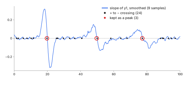
Chart 5. Smoothed slope $y'$ of $y_1$ (Math 3, window 9): 24 downward zero crossings, 3 kept as peaks
Advantages
- Fewer candidates: 24 against 116 before any filter.
- Shoulders visible: the slope of a shoulder dips toward zero without crossing it, a hint the local method never shows.
Disadvantages
- One more knob: too small a window and the noise returns; too large and narrow peaks are flattened away.
- Even spacing: the Savitzky-Golay slope assumes evenly spaced $x$.
Continuous Wavelet Transform
In plain words. Compare the signal at each position with a peak-shaped template—the Ricker wavelet—at several scales. A real peak often produces a strong response across several scales, whereas noise tends to match only at the smallest scales. Not always: a very narrow real peak may show only at small scales. The continuous wavelet transform (CWT) identifies positions whose responses persist across scales.
Control parameters. wmin and wmax set the
minimum and maximum template scales $a$ in Math 4, measured in samples (2 and 20 by
default). The local-method filters are then applied.
Basic idea. The Ricker wavelet of width $a$ and the transform at position $b$ (Math 4):
Math 4.
- Why many widths: one width either passes the noise (too small) or merges close peaks (too large). Asking for a match across a range of widths drops both failures.
- On $y_1$: Chart 6 draws $W(a, b)$ of $y_1$ from Chart 1 at three widths, 2, 8 and 20 samples. At width 2 the noise shows everywhere; at 8 and 20 only the three peaks stand out. The method identifies 7 candidates; the prominence filter retains 3.
- Ridges: the method follows each maximum of $W$ from width to width and keeps the ones whose ridge is long enough.
- Width $a$ is not FWHM: $a$ sets the template's scale. The peak it matches best is several $a$ wide; measure the width in stage 2.
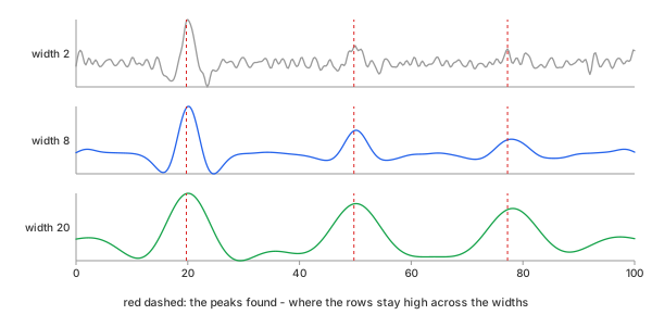
Chart 6. Wavelet transform $W(a, b)$ of $y_1$ (Math 4) at three widths $a$; the peaks found marked in red
Advantages
- Noise-robust: 7 candidates before any filter, the fewest of the three methods.
- No smoothing step: the range of widths does the smoothing.
Disadvantages
- Slow: a convolution is required at each scale; the advanced calculator therefore limits the input to 5,000 rows.
- Width range: peaks narrower than
wminor wider thanwmaxare missed. - Edges: near either end of the record the wavelet runs past the data, so $W$ there is distorted; a response at the very edge is not proof of a peak.
Stage 2, Measure: Width, Shape and Area
Half-Prominence Width
In plain words. A commonly used measure of peak width is the full width at half maximum (FWHM): the width halfway up from the peak's baseline. The half-prominence width (HPW) measures the width directly from the data: draw a horizontal line halfway down the peak's prominence, then measure the width of the peak at that level. It requires no peak-shape model. It equals the FWHM for a lone peak on a flat baseline.
Control parameters. None; the half height comes from the prominence of Math 2.
Basic idea. The half-prominence level is $y_h = y_i - P_i/2$. Starting from the peak, move outward until the data cross $y_h$ on each side. Use linear interpolation between the two samples surrounding each crossing to obtain $x_L$ and $x_R$ (Math 5):
Math 5.
- Why half the prominence: half the height above zero would depend
on the offset; half the prominence measures from the ground the peak stands on.
SciPy's
peak_widthsdoes the same withrel_height= 0.5. - When it departs from FWHM: a sloping baseline, bases of different heights, or a second peak in the flank. The ground is then not the peak's true baseline.
- On $y_1$: Chart 7 zooms on the first peak of $y_1$ from Chart 1. The peak height is 1.0888 and its prominence is $P$ = 1.0247, giving $y_h$ = 0.5765. The crossings are at 17.902 and 22.085: HPW = 4.18, against the true FWHM of 4.
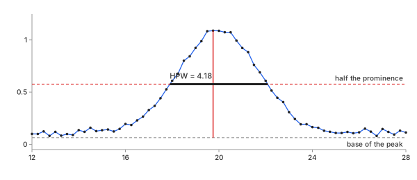
Chart 7. Half-prominence width (Math 5) of the first peak of $y_1$: 4.18 for a true FWHM of 4
Advantages
- Model-free: it assumes no shape, so it works on any single peak.
- Instant: no iteration, no start values.
Disadvantages
- Overlap: two merged peaks are measured as one wide one—52 % too wide in Chart 3, left.
- Noise at the crossing: one noisy sample near $y_h$ moves $x_L$ or $x_R$.
- Edges: a peak whose flank runs off the end of the record has no crossing there; its width is cut short.
- No area, no shape.
Peak Function Fit
In plain words. Represent each peak with a peak function—Gaussian, Lorentzian or Voigt—and adjust all peak functions simultaneously until their sum matches the data. Each fitted function then carries its own position, amplitude, width and area, even where the peaks overlap.
Control parameters. The number of peaks $N$, and per peak its
type, start position ($\mu$), start fwhm and start
amplitude ($A$). Stage
1 supplies the starts; the calculator's peaks select defaults to the number stage 1
found.
Basic idea. The three peak functions below have amplitude $A$, their height above the offset, and are centred at $\mu$. The Gaussian, from random broadening (Math 6):
Math 6.
The Lorentzian, which describes broadening associated with a finite lifetime and has heavy tails (Math 7):
Math 7.
The Voigt, which combines Gaussian and Lorentzian broadening through convolution and is scaled to have amplitude $A$ (Math 8):
Math 8.
Here $V$ is the unit-area Voigt profile, and $f_G = 2\sqrt{2\ln 2}\,\sigma$ and $f_L = 2\gamma$ are the widths of its two parts. Chart 8 draws the three shapes with the same amplitude 1 and the same FWHM of 4: they agree at the top and differ in the tails. At a distance of 6 from the centre, the Gaussian falls to 0.002, the Voigt to 0.062, and the Lorentzian to 0.100. So their areas differ: 4.26, 5.44 and 6.28.
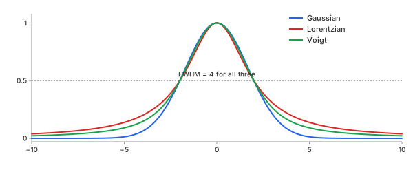
Chart 8. Gaussian (Math 6), Lorentzian (Math 7) and Voigt (Math 8) with the same amplitude and FWHM
The model for $N$ peaks includes a constant baseline offset $c$ and is fitted by least squares (Math 9):
Math 9.
- Why start values: the fit iteratively adjusts the parameters from their initial values. If an initial value is too far from the actual peak, the fit may converge to an incorrect solution. Stage 1 gives each peak a start at its position and HPW.
- On $y_1$: Chart 9 fits $y_1$ of Chart 1 with the three shapes it was made from. The input is the light black line, each peak function a green dashed line, their sum the bold red line. In 5 evaluations, the fit returns positions of 19.992, 50.010 and 78.019 (true values: 20, 50 and 78), amplitudes of 0.989, 0.697 and 0.499 above a baseline offset of 0.098, and widths of 4.02, 6.20 and 8.01.
- Amplitude and offset: the fitted amplitude $A$ is measured relative to the baseline offset $c$, whereas the stage 1 height is the raw value $y_i$.
- Bounds: $A \ge 0$ (a valley: $A \le 0$), each $\mu$ inside the $x$ range, each width above a twentieth of the smallest $x$ step. Without these bounds, the fit may use a positive peak and a negative peak to cancel part of each other. Their sum may still match the data, but the individual components would have no meaningful physical interpretation.
- Baseline: the baseline $c$ is constant. A sloping or curved baseline should either be removed first (remove the baseline) or be added to the model as its own term, such as $c_0 + c_1 x$; left in, it bends the peak parameters.
- Overlap: when peaks overlap, the fit can separate their individual contributions within the summed model; see the Example below.
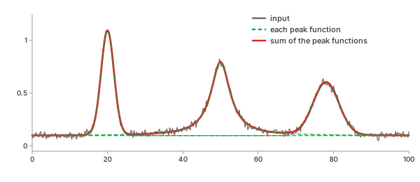
Chart 9. $y_1$ fitted with three peak functions (Math 9): input light black, each peak function green dashed, their sum red
Advantages
- Overlap: separates peaks that share one bump.
- Everything at once: sub-sample position and amplitude, width, shape and area, together with standard errors for the fitted parameters.
- Noise averaged: every sample under a peak helps fix its parameters.
Disadvantages
- A model: the shape and the number $N$ are choices; a wrong choice still returns numbers.
- Correlated parameters: where peaks overlap, the amplitude, width and position of neighbours trade off against each other. A small residual does not make each parameter reliable; read the standard errors. They hold only if the model is right: they assume the chosen shape, $N$ and noise, and say nothing about whether those choices are right.
- Start values: requires initial values from stage 1 or values supplied by the user.
- Slower: an iterative fit; the advanced calculator caps it at 5 seconds.
Which One Should You Choose?
For stage 1, Table 2 shows how many peaks each method detects in $y_1$ from Chart 1, both before filtering and after applying the default prominence threshold of 10 %. Chart 10 (left) plots these counts.
| method | no filter | prominence 10 % | use when |
|---|---|---|---|
| local maximum + filters | 116 | 3 | the default: exact, fast, one clear knob |
| derivative zero-crossing | 21 | 3 | evenly spaced data, shoulders worth a hint |
| continuous wavelet transform | 7 | 3 | heavy noise, peaks of known width range |
Table 2. Stage 1 methods on $y_1$: peaks found
The derivative method gives 21 peaks in this table but 24 zero crossings in Chart 5. After each crossing is assigned to its highest nearby sample, three crossings coincide with samples already assigned to neighbouring crossings. For stage 2, Table 3 compares the two methods on the larger peak of $y_2$; Chart 10, right, draws its widths.
| method | width | error | use when |
|---|---|---|---|
| true | 10.00 | — | |
| half-prominence width | 15.25 | +52 % | one peak alone, any shape |
| peak function fit, $N$ = 2 | 10.05 | +0.5 % | overlap, area, shape, error bars |
Table 3. Stage 2 methods on the larger peak of $y_2$: width (true and fit: FWHM)
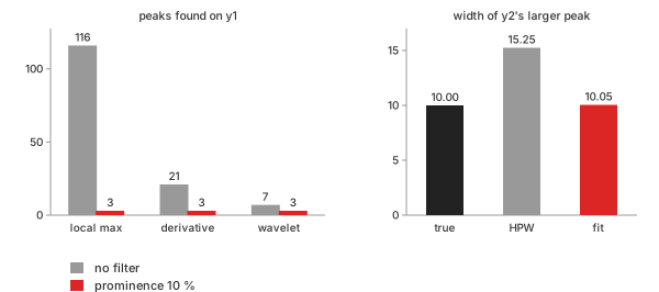
Chart 10. Left: peaks found on $y_1$ (Table 2). Right: width of the larger peak of $y_2$ (Table 3)
After filtering, all three methods identify the same three peaks. In this example, the choice of filter matters more than the detection method. Start with the local maximum and prominence; reach for the fit as soon as peaks overlap or the area is wanted.
Key Ideas
Height: An Absolute Threshold
A height filter keeps peaks whose top is above a fixed level. It is often the first filter people try, but it fails in this example. Chart 11 sets 0.65 on $y_1$ of Chart 1: it drops the noise, and it also drops the third peak, a real one, whose top is 0.638.
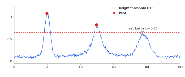
Chart 11. A height threshold of 0.65 on $y_1$ keeps two peaks and drops the third, real one
The height threshold depends on the baseline offset and overall data scale. Use it to reject peaks below a known detection limit, rather than as the primary means of identifying peaks.
Prominence: How Far a Peak Stands Out
Prominence (Math 2) separates the three real peaks from the 113 noise-induced maxima in Chart 4. Because it is measured relative to the surrounding bases, prominence is independent of a constant vertical offset. A small peak on the flank of a larger peak also retains its own prominence. As a fraction of the range, 10 % is a starting point, not a rule: the right value depends on the noise, the dynamic range and how small the wanted peaks are. One outlier or one very tall peak stretches the range; lower the limit for small peaks next to a tall one.
Distance: One Peak per Bump
A broad, noisy bump can contain many local maxima near its top. Without filtering, the region around the third peak of $y_1$ in Chart 1 ($x$ = 72 to 84) contains 14 local maxima. A distance setting of 40 samples (equivalent to 10 units of $x$) processes the maxima from highest to lowest and rejects any candidate that is less than 40 samples from an already retained peak. Only one remains, at $x$ = 77.25 (Chart 12).
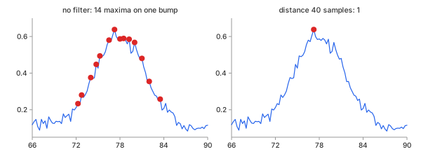
Chart 12. The third peak of $y_1$: 14 local maxima with no filter (left), 1 with a distance of 40 samples (right)
Distance is a blunt tool: of two real peaks closer than the limit, it drops the weaker. Prominence usually does the job without it.
Plateaus: Flat Tops
A saturated detector clips the top of a peak, producing a flat plateau. Math 1 then finds no strict maximum at all; the flat run must be treated as one peak. The plateau rule identifies a strict rise followed by a run of equal-valued samples, $y_l = \dots = y_r$, and then a strict fall. The peak is assigned to the middle sample of the plateau (Math 10).
Math 10.
When $l = r$, the plateau contains a single sample and the rule reduces to Math 1.
Chart 13 clips $y_1$ of Chart 1 at 0.8: the first peak develops a
plateau of 12 equal-valued samples from $x$ = 18.5 to 21.25. The
reported peak position is the middle sample, $x$ = 19.75. The
plateau filter sets a minimum flat-top size in samples.
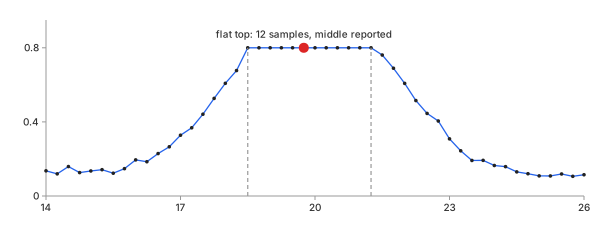
Chart 13. $y_1$ clipped at 0.8: a flat top of 12 samples, its middle reported as the peak
Clipping necessarily distorts a peak's measured height and width. Only a fit to the unclipped flanks can estimate the true top.
Valleys: Invert the Signal
An absorption spectrum or a transmission dip shows its features as valleys. Each method above can detect valleys by applying it to the inverted signal, $-y$. Chart 14 turns $y_1$ of Chart 1 into an absorption-like record, $1.2 - y_1$: the valleys are found at the same 19.75, 49.75 and 77.25, with depths 1.02, 0.74 and 0.55—the prominences of Chart 4.
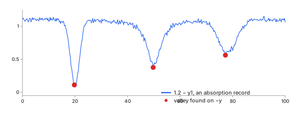
Chart 14. $1.2 - y_1$: the valleys, found on $-y$
Noise Invents Peaks
The 113 additional maxima in Chart 2 are caused by noise. Smoothing before the search cuts them down: a Savitzky-Golay smoother with a window of 21 samples leaves 46 local maxima on $y_1$ of Chart 1, against 116 (Chart 15). Smoothing alone does not reduce the count to three; the filters are still needed. A window that is too wide, however, would flatten the first and narrowest peak.
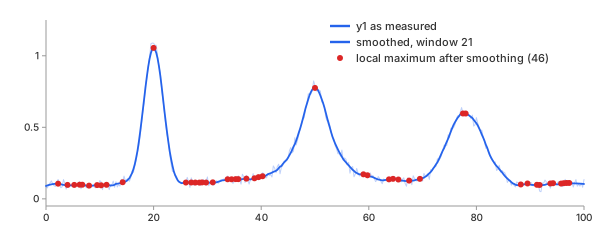
Chart 15. $y_1$ smoothed with a window of 21: 46 local maxima remain
A sloping or curved baseline can also cause problems: it raises the apparent peak levels on one side and changes their prominence. Remove the baseline first, then search.
Example: Two Overlapping Peaks
Return to $y_2$ of Chart 1: two Gaussians, 1.0 high at 46 and 0.6 high at 54, both 10 wide, 8 apart. Stage 1 detects one peak at $x$ = 47, with a raw height of 1.2369 and a half-prominence width of 15.25 (Chart 3, left). The shoulder has no maximum of its own.
Fit the data twice, using different numbers of peaks (Chart 16). With $N$ = 1, the fit returns a single Gaussian centred at 48.68 with a width of 14.42. It follows the middle of the bump but misses the data on both sides. The residual RMS is 0.0318, three times the noise standard deviation. With $N$ = 2, the initial values are obtained by splitting the stage 1 peak into two. The fit returns two Gaussians centred at 46.08 and 54.12, and the residual RMS decreases to 0.0099, close to the noise standard deviation of 0.01.
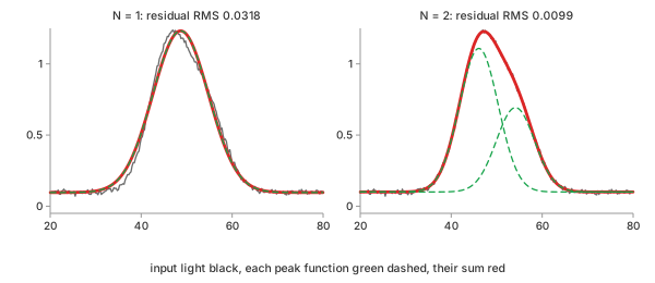
Chart 16. $y_2$ fitted with $N$ = 1 (left) and $N$ = 2 (right): input light black, each peak function green dashed, their sum red
Table 4 sets the results against the values $y_2$ was made from. The fitted amplitudes are measured above the fitted baseline offset of 0.100; stage 1 reports the raw height instead.
| position | amplitude | FWHM | area | |
|---|---|---|---|---|
| true, peak 1 | 46 | 1.0 | 10 | 10.645 |
| true, peak 2 | 54 | 0.6 | 10 | 6.387 |
| stage 1: HPW of the merged bump | 47 | 1.2369 (raw height) | 15.247 | — |
| fit $N$ = 1 | 48.675 | 1.1355 | 14.420 | 17.429 |
| fit $N$ = 2, peak 1 | 46.075 ± 0.103 | 1.0082 ± 0.0168 | 10.047 ± 0.109 | 10.782 ± 0.288 |
| fit $N$ = 2, peak 2 | 54.124 ± 0.171 | 0.5926 ± 0.0174 | 9.915 ± 0.179 | 6.255 ± 0.288 |
Table 4. $y_2$: true values against stage 1 and the two fits of Chart 16 (± one standard error)
Each value of the $N$ = 2 fit is within one standard error of its corresponding true value. This is an example of curve fitting with a model built from peaks; the residual RMS provides an initial guide to choosing $N$: add peaks while the residual RMS decreases toward the noise level, and stop when it reaches that level. This is not definitive evidence, because adding another peak will almost always reduce the residual. Also check that the residuals show no systematic pattern, that the added peak's standard errors remain small, and that the peak is physically meaningful. AIC and BIC balance the improvement in fit against the number of additional parameters.
Find the peaks with prominence, measure them with a fit. When the residual keeps a shape above the noise, a peak may be hiding, or the model does not fit.
REFs
Wikipedia, Full width at half maximum Wikipedia, Gaussian function Wikipedia, Cauchy distribution Wikipedia, Voigt profile SciPy scipy.signal.find_peaks SciPy scipy.signal.peak_prominences SciPy scipy.signal.peak_widths SciPy scipy.signal.find_peaks_cwt SciPy scipy.optimize.least_squares SciPy scipy.special.voigt_profile NIST/SEMATECH e-Handbook, Nonlinear Least Squares Regression Wikipedia, Topographic prominence Wikipedia, Ricker wavelet Smoothing Detrending Curve Fitting: Which Equation Fits My Data, and How Well?