An introduction to least-squares curve fitting: linear, polynomial, exponential, power-law, logarithmic, logistic, and Gaussian models; what R² and residual plots reveal; and how to recognize overfitting.
Contents
- What Is Curve Fitting? Which Equation Describes My Data?
- Least Squares: What Is Minimised
- Methods
- Which One Should You Choose?
- Key Ideas
- Polynomial Order: Too Low Misses, Too High Chases the Noise
- Goodness of Fit: R², Adjusted R², RMSE
- The Residual Plot Reads What R² Hides
- Linearised Fits: A Logarithm Changes the Answer
- Non-Linear Fits Need a Starting Guess
- Extrapolation: Where a Model Is Worst
- Standard Error: How Far a Coefficient Could Move
- REFs
What Is Curve Fitting? Which Equation Describes My Data?
A calibration run gives a sensor reading for each known concentration. A cooling experiment records the temperature every half-minute. A growth study records a count each day. In every case, the question is the same: which equation describes the data, what values should its coefficients have, and how well does it describe the observations?
Curve fitting provides a model: a formula with a few coefficients, such as $y = a + b\,x$, and the values of $a$ and $b$ that make it miss the data least. The model is the product; the fitted curve is only a picture of it. Two coefficients can stand for a hundred measured points, and they also give $y$ at an $x$ nobody measured.
This distinguishes curve fitting from two related methods (Fig 1). Interpolation passes through every point and treats each one as exact. Smoothing returns one cleaned value per point, but no formula. A fit misses points on purpose: it assumes the scatter is noise and keeps only the shape.
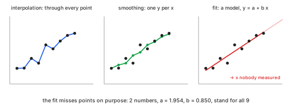
Fig 1. Interpolation joins the points, smoothing cleans them, a fit replaces them with an equation
Take an example: three columns measured at $x$ = 1, 1.5, 2, … 13—25 rows. The example has three purposes.
- $y_1$, a straight line. Made as $2 + 0.8\,x$ plus noise with a standard deviation of 0.4: the model is known, so a fit can be checked against it.
- $y_2$, a curve. Made as $1 + 2.2\,x - 0.16\,x^2$ plus the same noise: it rises, peaks near $x = 7$, and falls. A straight line cannot follow it.
- $y_3$, a decay. Made as $10\,e^{-0.3\,x}$ plus noise with a standard deviation of 0.2: a cooling curve or a discharge, falling from 7.39 to about 0.3.
Chart 1 shows all 25 rows of the three columns.
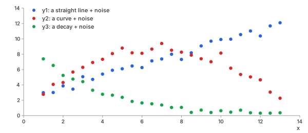
Chart 1. The example: a line, a curve, and a decay, each with noise
The task: recover the equation behind each column—and tell, from the data alone, when the equation is the wrong one.
Least Squares: What Is Minimised
A model $f(x)$ misses each point by its residual, the vertical distance between the measured $y_i$ and the model's value at the same $x_i$. Least squares picks the coefficients that make the sum of the squared residuals, SSE, as small as possible (Math 1):
Math 1.
Chart 2 shows the residuals of $y_1$ around its fitted line. Two choices hide in Math 1.
- Vertical: each residual is measured in $y$ only, not as the
shortest distance to the curve.
- assumes: all the error is in $y$, and $x$ is known exactly
- true for: a set concentration, a clock time, a chosen voltage
- not true for: two noisy measurements plotted against each other—that needs errors-in-variables methods, outside this page
- Squared: a residual twice as large costs four times as much.
- one far point: outweighs many near ones, and pulls the curve toward itself
- why squares: the minimum then has a closed form for every model that is linear in its coefficients
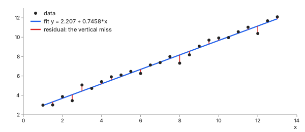
Chart 2. $y_1$ and its line: each residual is a vertical miss
Methods
The seven models fall into two groups (Fig 2). Linear, polynomial and logarithmic are linear in their coefficients: the minimum of Math 1 is found in one step, exactly. Exponential, power, logistic and Gaussian are not: the minimum is found by non-linear least squares, an iteration that starts from a guess.
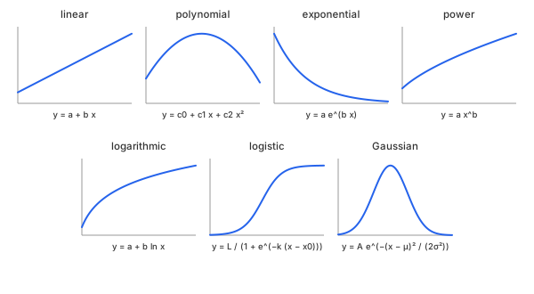
Fig 2. The seven model shapes
Linear
In plain words. A straight line: a constant slope, the same change in $y$ for every step in $x$. The simplest model, and the one every other model is compared with.
Control parameters. None: the model has two coefficients, $a$ and $b$, and both are fitted.
Basic idea. Simple linear regression. With the means $\bar{x}$ and $\bar{y}$, the minimum of Math 1 is (Math 2):
Math 2.
- Why use the means: the best line always passes through the point $(\bar{x}, \bar{y})$, so only its slope is left to find.
- Slope: how $x$ and $y$ move together, divided by how much $x$ moves on its own.
- If all $x$ values are the same: the denominator is 0, and no line is defined.
Example. Take the first five rows of $y_1$ (Table 1). The $x$ values add up to 10 and the $y$ values to 18.39, so $\bar{x} = 2$ and $\bar{y} = 3.678$.
| $x$ | $y_1$ | $x - \bar{x}$ | $y_1 - \bar{y}$ | $(x - \bar{x})(y_1 - \bar{y})$ | $(x - \bar{x})^2$ |
|---|---|---|---|---|---|
| 1 | 2.99 | −1.0 | −0.688 | 0.6880 | 1.00 |
| 1.5 | 3.01 | −0.5 | −0.668 | 0.3340 | 0.25 |
| 2 | 3.87 | 0.0 | 0.192 | 0.0000 | 0.00 |
| 2.5 | 3.45 | 0.5 | −0.228 | −0.1140 | 0.25 |
| 3 | 5.07 | 1.0 | 1.392 | 1.3920 | 1.00 |
| sum | 2.3000 | 2.50 | |||
Table 1. The first five rows of $y_1$, the two sums of Math 2
Then (Math 3):
Math 3.
The line $y = 1.838 + 0.92\,x$ misses the five points by 0.2320, −0.2080, 0.1920, −0.6880 and 0.4720; their squares add up to SSE = 0.8301. Over all 25 rows, the same formulas give $y = 2.207 + 0.7458\,x$ (Chart 2), close to the $2 + 0.8\,x$ the data were made from.
Important characteristics. One closed-form step, no starting guess, always the same answer.
Advantages
- Exact, fast, and needs no guess.
- Both coefficients have a plain meaning: the value at $x = 0$, and the change per unit of $x$.
Disadvantages
- Only a straight line: on $y_2$, it finds almost nothing (R² 0.0113).
- Squared residuals: one far point tilts the whole line.
Polynomial
In plain words. A straight line plus powers of $x$: $x^2$ adds one bend, $x^3$ a second, and so on. The order sets how many bends the curve may have—and every extra order is one more coefficient to fit.
Control parameters. order ($n$ below, default 2, from 1
to 10): the highest power of $x$. The model has $n + 1$ coefficients; order 1 is the
linear model.
Basic idea. Polynomial regression (Math 4):
Math 4.
- Why it still takes only one step: $f$ is a sum of known functions
of $x$ ($1, x, x^2, \dots$), each times a coefficient, so it is linear in the
coefficients and Math 1 has one exact minimum—a single least-squares solve, as
numpy.polyfitdoes. - Required number of points: at least $n + 1$ points, at $n + 1$ different $x$ values.
- With exactly $n + 1$ points: the curve passes through every one—this is interpolation, not a fit (see Polynomial Order).
Example. $y_2$ at order 2 gives $y = 0.803361 + 2.31723\,x - 0.169773\,x^2$, with R² 0.9604—against 0.0113 for the straight line, which cannot bend (Chart 3). The data were made from $1 + 2.2\,x - 0.16\,x^2$.
Important characteristics. A polynomial can be flexible near the data but unreliable outside the measured range, because its highest powers can grow without bound.
Advantages
- Exact and fast, like the line, and follows almost any smooth shape.
- One knob, the order, sets the flexibility.
Disadvantages
- Too high an order chases the noise (see Polynomial Order).
- Outside the data, high powers run away (see Extrapolation).
- The coefficients rarely mean anything physical.
Exponential
In plain words. Constant relative change: each step in $x$ multiplies $y$ by the same factor. Growth when $b > 0$, decay when $b < 0$—cooling, discharge, radioactive decay, compound interest.
Control parameters. space (advanced calculator):
non-linear, the default, minimises Math 1 on $y$ itself; linearised fits a straight
line to $\ln y$ instead (see Linearised Fits).
Basic idea. With $a$ the value at $x = 0$ and $b$ the rate (Math 5):
Math 5.
- Why iteration is needed: $b$ sits inside the exponential, so
Math 1 has no closed-form minimum.
scipy.optimize.curve_fitstarts from a guess and improves it step by step (the Levenberg–Marquardt algorithm). - Starting guess: from the linearised fit, when every $y > 0$.
- Half-life: for a decay, $y$ halves every $\ln 2 / |b|$.
Example. $y_3$ gives $y = 9.928\,e^{-0.295743\,x}$, R² 0.9928, close to the $10\,e^{-0.3\,x}$ it was made from; the half-life is $0.6931 / 0.2957 = 2.34$.
Important characteristics. Never crosses zero; the curve keeps the sign of $a$.
Advantages
- Two coefficients with a physical meaning: start value and rate.
- The natural model of every process whose rate is proportional to its size.
Disadvantages
- No offset: a decay toward a nonzero level (room temperature) leaves a pattern in the residuals.
- Iterative: needs a starting guess, and can fail (see Starting Guess).
Power Law
In plain words. Constant relative change per relative change: doubling $x$ always multiplies $y$ by the same factor. Area against length, drag against speed, metabolic rate against body mass—a power law is a straight line on a log–log plot.
Control parameters. space, as for the exponential:
non-linear, or a straight line through $(\ln x, \ln y)$.
Basic idea. With $b$ the exponent (Math 6):
Math 6.
- Why $x > 0$ is required: $x^b$ of a negative $x$ is not a real number for most $b$, and $\ln x$ does not exist; the calculator refuses such a column, naming it.
- Doubling: doubling $x$ multiplies $y$ by $2^b$.
Example. $y_1$ gives $y = 2.14011\,x^{0.65642}$, R² 0.9731—lower than the straight line's 0.9824. A power law with $b < 1$ bends over, and the line in $y_1$ does not.
Important characteristics. Passes through $(0, 0)$ when $b > 0$: no offset.
Advantages
- The exponent $b$ is often the quantity of interest (a scaling law).
- Covers lines ($b = 1$), parabolas ($b = 2$), and roots ($b = 0.5$) with one model.
Disadvantages
- Only $x > 0$.
- No offset: data that start from a nonzero $y$ at $x = 0$ do not fit.
Logarithmic
In plain words. Constant change per relative change: each doubling of $x$ adds the same amount to $y$. Steep at first, then ever slower, and never leveling off completely—loudness in decibels, the pH scale, learning curves.
Control parameters. None.
Basic idea. A straight line in $\ln x$ (Math 7):
Math 7.
- Why it takes one step: $f$ is linear in $a$ and $b$; with $u = \ln x$ it is the line of Math 2, so the fit is exact.
- Doubling: doubling $x$ adds $b \ln 2$ to $y$.
Example. $y_3$ gives $y = 7.22275 - 2.90895 \ln x$, R² 0.9740: a falling curve that flattens, but less well than the exponential's 0.9928.
Important characteristics. Unbounded in both directions: no plateau.
Advantages
- Exact, no guess.
- The natural model when $y$ responds to ratios of $x$.
Disadvantages
- Only $x > 0$.
- Data that truly level off (a plateau) leave a pattern in the residuals.
Logistic (Sigmoid)
In plain words. An S-curve: slow start, rapid middle, and a plateau it never passes. Population growth with limited resources, a dose–response curve, the spread of an adoption.
Control parameters. None to set: the three coefficients are fitted from an automatic starting guess.
Basic idea. The logistic function, with the plateau $L$, the steepness $k$ and the midpoint $x_0$ (Math 8):
Math 8.
- Why three coefficients are needed: height ($L$), position ($x_0$, where $y = L/2$) and width (the rise from 10% to 90% of $L$ takes $4.39 / k$).
- Starting guess: $L$ from the largest $y$, $x_0$ from where the data cross half of it, the sign of $k$ from the trend.
Example. $y_1$ gives $L = 15.4927$, $k = 0.207324$, $x_0 = 7.44603$, R² 0.9800—almost as good as the straight line, because 25 points of a line also look like the lower half of an S. The plateau of 15.49 lies above every measured value: the model predicts it, the data never showed it. On $y_3$ the fit reaches R² 0.9928 with $L = 473113$, a plateau that means nothing.
Important characteristics. A coefficient is only meaningful if the data cover the feature it describes: $L$ needs the plateau, $x_0$ the midpoint.
Advantages
- Bounded: the curve can never run past its plateau.
- Each coefficient is a readable feature of the curve.
Disadvantages
- Data that do not show both ends leave $L$ or $x_0$ poorly defined—a high R² hides it.
- Iterative, three coefficients, a guess needed.
Gaussian Peak
In plain words. A symmetric bell: one peak, falling to zero on both sides. A spectral line, a chromatography peak, a beam profile.
Control parameters. None to set: the three coefficients are fitted from an automatic starting guess.
Basic idea. The Gaussian function, with the height $A$, the center $\mu$ and the width $\sigma$ (Math 9):
Math 9.
- Why use a peak model: the center $\mu$ and the width are usually what is measured—a wavelength, a retention time, a beam size.
- Width: the full width at half maximum is $2.355\,\sigma$.
- Starting guess: $A$ and $\mu$ from the largest point, $\sigma$ from the width where the data stay above half of it.
Example. $y_2$, a hump, gives $A = 8.94966$, $\mu = 6.77743$, $\sigma = 4.20695$, R² 0.9395—lower than the parabola's 0.9604: the hump of $y_2$ is a parabola, with no tails falling toward zero. On $y_3$, which has no peak, the solver does not converge, and the calculator reports that instead of a curve.
Important characteristics. Falls to zero on both sides: no baseline.
Advantages
- Center, height and width read straight off the coefficients.
- The standard shape of a peak broadened by many small random effects.
Disadvantages
- A peak on a sloping or offset background needs that background removed first—detrending.
- Overlapping peaks need a sum of Gaussians - peak fitting.
The Seven Side by Side
Each model fitted to each data column (Table 2; polynomial at order 2):
| model | $y_1$ (line) | $y_2$ (curve) | $y_3$ (decay) |
|---|---|---|---|
| linear | 0.9824 (0.3601) | 0.0113 (2.0099) | 0.8080 (0.8865) |
| polynomial | 0.9824 (0.3601) | 0.9604 (0.4020) | 0.9794 (0.2904) |
| exponential | 0.9588 (0.5508) | 0.0089 (2.0124) | 0.9928 (0.1714) |
| power | 0.9731 (0.4449) | 0.0264 (1.9945) | 0.9131 (0.5963) |
| logarithmic | 0.8894 (0.9022) | 0.0336 (1.9872) | 0.9740 (0.3261) |
| logistic | 0.9800 (0.3838) | 0.4191 (1.5406) | 0.9928 (0.1714) |
| Gaussian | 0.9801 (0.3825) | 0.9395 (0.4973) | no convergence |
Table 2. R² (with RMSE in parentheses) for each model and data column; the model used to generate each column is in bold
The true model has the best R² in each column—but by small margins, and not alone: on $y_1$, the order-2 polynomial ties the line (its $x^2$ coefficient is −0.0000290), and on $y_3$, the logistic ties the exponential with a meaningless plateau. R² alone cannot choose a model; the next sections show what can.
Which One Should You Choose?
| your data | use | in the example |
|---|---|---|
| a constant rate of change, a calibration line | linear | $y_1$: 0.9824 |
| a smooth curve, no physical model, used inside the data range | polynomial, lowest order that leaves no pattern | $y_2$: order 2, 0.9604 |
| growth or decay at a rate proportional to the size | exponential | $y_3$: 0.9928 |
| a scaling law, straight on a log–log plot | power law | — |
| a response to ratios of $x$, slowing without a limit | logarithmic | — |
| an S-curve with a visible plateau | logistic | — |
| a single symmetric peak on a flat zero baseline | Gaussian | — |
Table 3. Choose a model by the process that generated the data, not by the highest R²
Start from what produced the data. A physical model—decay, growth, a scaling law—has coefficients that mean something and that hold outside the data. A polynomial is a description, valid only where it was fitted. In either case, check the residual plot before believing the fit.
Key Ideas
Polynomial Order: Too Low Misses, Too High Chases the Noise
Chart 3 fits $y_2$ at three orders. Order 1 is a straight line fitted to a hump: it misses the shape entirely (R² 0.0113). Order 2 follows the hump. Order 10 follows it too, with nine more coefficients, and bends toward single noisy points—R² rises only from 0.9604 to 0.9644.
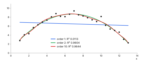
Chart 3. $y_2$ at orders 1, 2 and 10: order 1 misses the shape, order 10 adds nothing but wiggles
At the extreme, an order of $N - 1$ through $N$ points has as many coefficients as there are points, and passes through every one of them. Chart 4 takes seven points of $y_2$, every fourth row, and fits order 6: every residual is 0, R² is 1, and the curve overshoots to 9.535 between the points. It is no longer a fit at all; it is polynomial interpolation. Order 2 through the same seven points stays close to the curve the data came from.
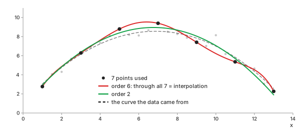
Chart 4. Seven points, order 6: through every point, which is interpolation, not a fit
This is the bias–variance trade: too few coefficients and the model is wrong everywhere (bias); too many and it follows this particular noise, and would follow different noise in a repeat measurement (variance).
Goodness of Fit: R², Adjusted R², RMSE
Three numbers summarise a fit, with $\bar{y}$ the mean of the data and $p$ the number of coefficients (Math 10):
Math 10.
- Why a reference: SSE alone has the units of $y^2$ and grows with $N$; it needs something to compare with.
- R²:
SSE against SST, the squared misses of a flat line at the mean.
- 1: every point on the curve
- 0: no better than the mean
- below 0: worse than the mean—possible only for a non-linear model, a sign the solver failed
- Adjusted R²: charges for each coefficient; it falls when a new one does not earn its place. Undefined when $N = p$.
- RMSE: the typical miss, in the units of $y$.
Example. For the five points of Table 1, SST = 2.9461 and SSE = 0.8301 (Math 11):
Math 11.
Table 4 fits $y_2$ at every order from 1 to 10.
| order | R² | adjusted R² | RMSE |
|---|---|---|---|
| 1 | 0.0113 | −0.0317 | 2.0099 |
| 2 | 0.9604 | 0.9568 | 0.4020 |
| 3 | 0.9616 | 0.9562 | 0.3959 |
| 4 | 0.9620 | 0.9544 | 0.3939 |
| 5 | 0.9630 | 0.9532 | 0.3889 |
| 6 | 0.9630 | 0.9507 | 0.3887 |
| 7 | 0.9631 | 0.9479 | 0.3882 |
| 8 | 0.9631 | 0.9447 | 0.3882 |
| 9 | 0.9632 | 0.9411 | 0.3878 |
| 10 | 0.9644 | 0.9390 | 0.3813 |
Table 4. $y_2$ at polynomial orders 1 to 10: R² never decreases, while adjusted R² peaks at order 2
R² rises at every order, because a model with one more coefficient can always do at least as well; it cannot choose an order. Adjusted R² peaks at order 2—the order the data were made from—and falls after. RMSE at order 2, 0.4020, is the noise put into the data, 0.4: there is nothing left to explain. Report RMSE alongside R²: an R² of 0.96 does not tell you whether the typical miss is 0.4 or 400.
The Residual Plot Reads What R² Hides
A straight line through $y_3$ has R² 0.8080—respectable on its own. Its residuals, plotted against $x$, tell a different story (Chart 5): the first five are positive, the next thirteen negative, the last seven positive again. A U-shape is curvature the model did not capture. The exponential leaves residuals that change sign at random: noise, and nothing else.
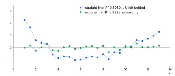
Chart 5. Residuals of $y_3$: the straight line leaves a U, the exponential leaves noise
The rule is simple: a pattern in the residuals suggests that the model is wrong, regardless of how high R² is. A good fit leaves residuals with no visible pattern—no curve, no trend, no spread that grows with $x$. The NIST e-Handbook builds its whole model check on this plot.
Linearised Fits: A Logarithm Changes the Answer
Taking the logarithm turns an exponential into a straight line, and a straight line can be fitted in one exact step (Math 12):
Math 12.
It is not a shortcut to the same answer. Fitting $\ln y$ minimises the squared misses in $\ln y$—relative errors—while Math 1 minimises the misses in $y$. On $y_3$, the two disagree (Chart 6):
- Non-linear: $y = 9.928\,e^{-0.295743\,x}$, RMSE 0.1714.
- Linearised: $y = 8.82551\,e^{-0.272799\,x}$, RMSE 0.2656.
- Why: at $x = 13$, $y_3 = 0.37$, and noise of 0.2 is half the value; at $x = 1$, $y_3 = 7.39$, and the same noise is under 3% of it. In $\ln y$, the small values at the end weigh as much as the large ones at the start, so the linearised line follows the tail and misses the first points by 0.672 and 0.678.
- Domain: $\ln y$ needs every $y > 0$; one zero or negative reading and the linearised fit is impossible.
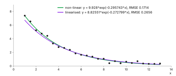
Chart 6. $y_3$: the non-linear and the linearised exponential are two different fits
Which is right depends on the noise. If the noise is a fixed amount, as in $y_3$, the non-linear fit is the honest one. If it is a fixed percentage—counts, concentrations over several decades—the linearised fit weighs the points correctly. The advanced calculator offers both and names which one ran.
Non-Linear Fits Need a Starting Guess
An iterative solver walks downhill on SSE from where it starts. From a good start it finds the minimum; from a bad one it can stop somewhere else, or not stop at all. Chart 7 fits a Gaussian to $y_2$ twice.
- Automatic guess: $A = 9.4$, $\mu = 7$, $\sigma = 3.822$, from the largest point → $\mu = 6.77743$, R² 0.9395, after 17 evaluations.
- Peak placed at $x = 20$: $\sigma = 1$, outside the data. The model is below $2 \times 10^{-10}$ at every point, so moving any coefficient changes nothing, and the solver stops after 25 evaluations exactly where it started: R² −10.334.
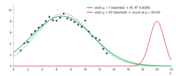
Chart 7. A Gaussian on $y_2$: from the automatic guess the solver finds the hump; from $\mu = 20$ it never moves
The second run "converged": the solver reported success. A fit should be checked rather than trusted. The calculator rejects a non-linear result that does worse than a flat line (R² below 0). If a fit fails to converge, as the Gaussian fit to $y_3$ does in Table 2, the calculator reports the failure instead of returning a misleading curve. And a converged fit can still be meaningless, as the logistic plateau of 473113 on $y_3$ shows.
Extrapolation: Where a Model Is Worst
A model gives $y$ at any $x$, including those outside the data. Interpolation stops at the last point; a fit cannot refuse, so it must be read with care. Chart 8 fits $y_2$ at orders 2 and 8. Inside the data the two are the same curve—R² 0.9604 and 0.9631. At $x = 20$, seven units past the last point, order 2 gives −20.76 and order 8 gives +157.94; the curve the data came from gives −19.00.
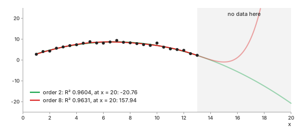
Chart 8. $y_2$ at orders 2 and 8: the same inside the data, opposite directions outside it
Extrapolation is safe only as far as the model is known to hold. A physical model (decay, growth) carries its reason with it; a polynomial carries none, and its highest power takes over as soon as the data stop holding it.
Standard Error: How Far a Coefficient Could Move
Fitted coefficients come from noisy data, so they are noisy too. The standard error of each coefficient says how far it would typically move if the measurement were repeated with new noise. With $J$ the matrix of the model's derivatives with respect to each coefficient, one row per point, and $s^2 = \mathrm{SSE} / (N - p)$ the residual variance (Math 13):
Math 13.
- Why $N - p$: $p$ coefficients fitted to $N$ points leave $N - p$ independent misses; $N = p$ leaves none, and no standard error.
- Reading it: roughly 95% of repeated measurements give a coefficient within two standard errors of the true value.
Example. $y_3$, exponential: $a = 9.9280 \pm 0.2168$ and $b = -0.2957 \pm 0.0074$. The values the data were made from, 10 and −0.3, lie 0.33 and 0.58 standard errors away. For $y_2$ at order 2, the intercept is $c_0 = 0.8034 \pm 0.3253$—a wide range, because $c_0$, $c_1$ and $c_2$ can trade off against each other: a little more of one, a little less of another, and the curve barely changes. That trade-off is the subject of parameter correlation, a topic of its own. The advanced calculator shows the standard error of every coefficient.
A fit is a model, not a curve that must pass through every point. Choose the model by the process behind the data, then check it with the residuals.
REFs
NIST/SEMATECH e-Handbook, Process Modeling NIST/SEMATECH e-Handbook, How can I tell if a model fits my data? NumPy numpy.polyfit SciPy scipy.optimize.curve_fit Wikipedia, Curve fitting Wikipedia, Least squares Wikipedia, Simple linear regression Wikipedia, Polynomial regression Wikipedia, Non-linear least squares Wikipedia, Levenberg–Marquardt algorithm Wikipedia, Coefficient of determination Wikipedia, Overfitting Interpolation Methods Smoothing Methods: Moving Average, EWMA, Savitzky-Golay, Gaussian, Median