How the inverse Fourier transform turns amplitudes over frequency back into samples over time - the inverse discrete Fourier transform (IDFT) that defines it, the inverse fast Fourier transform (IFFT) that computes it fast, and the five things that decide what comes out.
Contents
What is the inverse Fourier transform: what time signal does this spectrum make
You have a spectrum - a list of frequencies, each with an amplitude and a phase. It may be the output of an FFT, a spectrum you edited to remove a tone, or a specification written as "1 Hz at 1.0, 3 Hz at 0.5". The question this page answers is the reverse of the Fourier transform's: what signal over time does this spectrum make?
The inverse Fourier transform builds that signal. Every frequency in the spectrum becomes one wave - its height set by the amplitude, its starting point set by the phase - and the waves are added sample by sample. Nothing is estimated: if the spectrum came from an FFT, the samples come back exactly (Fig 1).
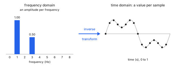
Fig 1. From frequency to time: the same data before and after the inverse transform
Take an example: the spectrum the Fourier transform page found in its own data. Sixteen bins, one second of record, so bin $k$ sits at $k$ Hz. Two of them are non-zero: 1.0 at 1 Hz and 0.5 at 3 Hz, both with phase $-\pi/2$ (Table 1).
| bin k | f (Hz) | amplitude | phase (rad) |
|---|---|---|---|
| 0 | 0 | 0.00 | 0 |
| 1 | 1 | 1.00 | −1.5708 |
| 2 | 2 | 0.00 | 0 |
| 3 | 3 | 0.50 | −1.5708 |
| 4 | 4 | 0.00 | 0 |
| 5 | 5 | 0.00 | 0 |
| 6 | 6 | 0.00 | 0 |
| 7 | 7 | 0.00 | 0 |
| 8 | 8 | 0.00 | 0 |
Table 1. The example: a one-sided spectrum, bins 0 to N/2 for N = 16
The bold rows are the two tones. A phase of $-\pi/2$ is a quarter turn behind a cosine, which is exactly a sine. Chart 1 draws the same table.
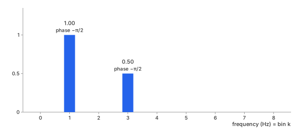
Chart 1. The spectrum of Table 1: amplitude per bin, phase above each bar
And Chart 2 is the signal it makes: the two waves, and their sum at every one of the 16 samples. The sum is the signal of the Fourier transform page's Table 1, to within $3 \times 10^{-15}$ - floating-point round-off and nothing else.
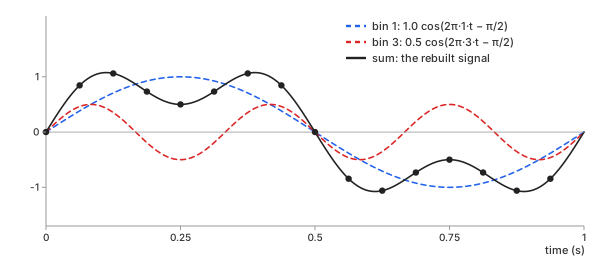
Chart 2. The signal Table 1 makes: the two waves and their sum at every sample
Getting from Chart 1 to Chart 2 is the whole job. The rest of this page is how it is done, how to do it fast, and the five things that decide what comes out.
Methods
Two routes, one answer. The IDFT is the definition, computed term by term. The IFFT is the forward FFT used a second time, with two sign flips and a division. On this data they agree to within $5 \times 10^{-15}$.
IDFT (direct sum)
In plain words. For every sample you want, go through the spectrum bin by bin: make that bin's wave, read its value at this sample, and add it to the total. The total is the sample.
Basic idea. With $N$ complex bins $Y_0, \dots, Y_{N-1}$, the inverse discrete Fourier transform gives each sample $y_n$ (Math 1). It is the forward DFT with the sign of the exponent flipped and a $1/N$ in front:
Math 1.
Math 1 wants all $N$ complex bins. Table 1 gives only bins 0 to $N/2$, as an amplitude $A_k$ and a phase $\varphi_k$. Each one becomes a complex bin, and the upper half is filled in as the mirror - the complex conjugate - of the lower half (Math 2):
Math 2.
The $N/2$ undoes the doubling the Fourier transform page applied to a one-sided spectrum, so a bin reading $A$ becomes a wave of height $A$. On the example (Math 3):
Math 3.
With the mirror in place, each pair $Y_k$, $Y_{N-k}$ adds up to one real cosine, and Math 1 becomes a plain sum of cosines (Math 4):
Math 4.
Here is one sample by hand: $n = 2$, at $t = 0.125$ s. Only bins 1 and 3 are non-zero (Math 5):
Math 5.
1.061 is row 2 of the Fourier transform page's Table 1. The other 15 samples work the same way (Table 2).
| n | t (s) | y |
|---|---|---|
| 0 | 0.0000 | 0.000 |
| 1 | 0.0625 | 0.845 |
| 2 | 0.1250 | 1.061 |
| 3 | 0.1875 | 0.733 |
| 4 | 0.2500 | 0.500 |
| 5 | 0.3125 | 0.733 |
| 6 | 0.3750 | 1.061 |
| 7 | 0.4375 | 0.845 |
| 8 | 0.5000 | 0.000 |
| 9 | 0.5625 | -0.845 |
| 10 | 0.6250 | -1.061 |
| 11 | 0.6875 | -0.733 |
| 12 | 0.7500 | -0.500 |
| 13 | 0.8125 | -0.733 |
| 14 | 0.8750 | -1.061 |
| 15 | 0.9375 | -0.845 |
Table 2. The rebuilt signal: all 16 samples, plotted in Chart 2
Important characteristics. Each of the $N$ samples needs a sum over all $N$ bins, so the IDFT costs $N^2$ complex multiplications - the same as the forward DFT.
Advantages
- It is the definition - every sample traces back to one visible sum
- Works for any $N$
- You can compute only the samples you need, one at a time
Disadvantages
- $N^2$ cost: 1,024 bins already need about a million multiplications
- Repeats the same products across different samples
IFFT (the forward FFT reused)
In plain words.
- Flip the sign of every bin's imaginary part (conjugate)
- Run the ordinary forward FFT on it
- Flip the signs again
- Divide by $N$
No separate inverse algorithm is needed: the fast FFT does all the work (Fig 2).
spectrum Y
    ↓
conjugate every bin
    ↓
forward FFT
    ↓
conjugate again, divide by N
    ↓
signal y
Fig 2. The IFFT as the forward FFT reused
Basic idea. Conjugating flips the sign of $i$. The forward FFT multiplies by $e^{-2\pi i k n/N}$; with the spectrum conjugated before and the result conjugated after, that sign comes out as the $+$ Math 1 needs (Math 6):
Math 6.
On the example, this route gives Table 2 again: the largest difference from the direct IDFT is $5 \times 10^{-15}$.
Important characteristics. The work is one forward FFT, so the cost is $\tfrac{N}{2}\log_2 N$ complex multiplications. The two conjugations and the division are $N$ cheap steps each.
Advantages
- Much faster than the direct IDFT, and the gap grows with $N$
- Exactly the same result as the IDFT
- Any FFT library already contains it
Disadvantages
- All $N$ samples or none: no single sample on its own
- Inherits every FFT detail - reordering, factorizations of $N$
Which one should you pick
For real data, the IFFT - the saving is the same as the forward one (Table 3).
| N | IDFT: $N^2$ | IFFT: $\tfrac{N}{2}\log_2 N$ |
|---|---|---|
| 16 | 256 | 32 |
| 1,024 | 1,048,576 | 5,120 |
| 65,536 | 4,294,967,296 | 524,288 |
Table 3. Cost in complex multiplications
The IDFT earns its place when you are learning what the inverse does, and when you need a few samples rather than the whole record. That is why the basic calculator runs an IDFT in your browser, and the advanced calculator offers the IFFT.
Key ideas
The inverse itself is exact. What decides the result is what you feed it - five things, each a common way to get a wrong signal from a right spectrum.
Round trip: FFT, then IFFT, returns the samples
Round trip - take samples, transform them, invert the result. You get the samples back, to round-off (Table 4):
| N | largest |IFFT(FFT(y)) − y| |
|---|---|
| 16 | 2.2 × 10⁻¹⁶ |
| 1,000 | 1.3 × 10⁻¹⁵ |
| 1,024 | 9.3 × 10⁻¹⁶ |
Table 4. Round trip on random data
That is the reason to edit a signal in the frequency domain: transform, change some bins, invert. Every bin left alone comes back untouched.
Scaling: where the 1/N sits
Scaling convention - the forward and inverse transforms together must divide by $N$ once. $N$ is the number of samples, which is also the number of bins in the full spectrum. In the example $N = 16$: one second at 16 samples per second gives 16 samples, and its full spectrum has 16 bins (Table 1 shows the 9 of them from 0 to $N/2$). So the inverse divides by 16 (Math 1); forget it and every sample comes back 16 times too big.
Libraries disagree on where the division goes: NumPy and SciPy put the whole $1/N$ on the inverse, the "ortho" convention puts $1/\sqrt{N}$ on each side. Mix two conventions and the signal comes back the wrong size (Table 5):
| what was done | peak of the example |
|---|---|
| NumPy default: $1/N$ on the inverse | 1.0607 (correct) |
| $1/N$ forgotten | 16.9706 (16×) |
| NumPy's spectrum inverted with "ortho" scaling | 4.2426 (4×) |
Table 5. One spectrum, three scalings
A result off by exactly $N$ or $\sqrt{N}$ is a scaling mismatch, never a wrong spectrum. The calculators on this site read amplitudes in the Fourier transform page's scale (Math 2), so its output inverts here unchanged.
Conjugate symmetry: mirror a one-sided spectrum first
Conjugate symmetry - a real signal has a spectrum whose upper half is the mirror of the lower: each upper bin is the complex conjugate of its partner, $Y_{N-k} = \overline{Y_k}$. Feed only the lower half to the inverse, with zeros above, and the result is complex (Chart 3):
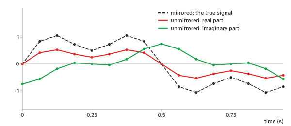
Chart 3. The example inverted without the mirror: half-height real part, a spurious imaginary part
The real part is exactly half the true signal, and the imaginary part reaches 0.75. Neither is a fault of the inverse: half the spectrum was missing. One-sided input - the usual output of a spectrum analyser or of the Fourier transform page - is mirrored first, as in Math 2.
Phase: same amplitudes, a different signal
Phase - where in its cycle each wave starts. Amplitudes alone do not fix the signal. Chart 4 keeps Table 1's amplitudes and changes only the two phases:
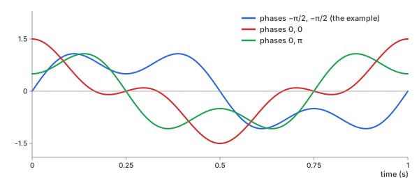
Chart 4. Table 1's amplitudes with three phase sets
Three different signals. With both phases 0 the two peaks line up and the signal reaches 1.5; the example's phases keep it to 1.0758. A spectrum given as amplitudes only - a magnitude plot, a datasheet curve - cannot be inverted to the one signal it came from. The phase has to be known too.
Zero-padding the spectrum: a finer time grid
Zero-padding - add bins of zero above the highest frequency, then invert. The record length stays one second, but there are more samples in it: 64 bins give 64 samples, four times finer (Math 7, Chart 5). Every bin keeps its value, scaled by $M/N$ so the amplitudes stay the same:
Math 7.
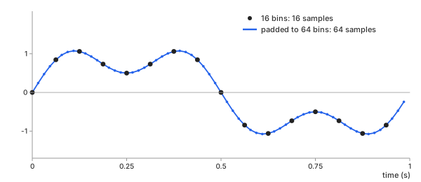
Chart 5. The example padded from 16 to 64 bins: four times the samples, the same signal
Every fourth new sample equals an original one, to $2 \times 10^{-14}$, and the rest fall on the true curve between them. It is interpolation that adds no new frequency - exact for a signal like this one, whose tones sit on the bins. For other ways to fill in between samples, see the interpolation page.
REFs
Fourier Transform (DFT, FFT): What Frequencies Are in My Data? - the forward half of this page Wikipedia, Discrete Fourier transform - inverse transform NumPy numpy.fft - normalization modes SciPy scipy.fft J. O. Smith, Mathematics of the Discrete Fourier Transform (DFT)