How to calculate the slope and area from measured x/y data: finite differences, Savitzky-Golay, trapezoid and Simpson rules, noise, step size and uneven x.
Contents
What Are a Numerical Derivative and Integral? Slope and Area from Numbers
A position recorded every tenth of a second, a power reading from a meter, or a current trace from a detector: each is a set of numbers, not a formula. Yet the questions are the same ones calculus answers. How quickly does the value change at each point (the derivative, or slope)? How much accumulates over a range (the integral, or area under the curve)? For example, velocity comes from position, energy from power, and charge from current.
With a formula, both operations follow directly from calculus rules: the derivative of $\sin x$ is $\cos x$. Measured data, however, provide no formula to differentiate or integrate. A numerical derivative is calculated from differences between the available values; a numerical integral is calculated by summing contributions across the data range. Their outputs have different units from the original $y$: the derivative has units of $y$ per $x$, while the integral has units of $y$ multiplied by $x$. To estimate the value of $y$ between two samples, see interpolation instead.
Consider three data columns, each sampled at 101 points from $x$ = 0 to 10 with a step size of $h$ = 0.1. Chart 1 and Chart 2 show the data, and Table 1 lists ten representative rows.
- $y_1 = \sin x$: clean, rounded to four decimals. Its true derivative, $\cos x$, and its true integral from 0, $1 - \cos x$, are known, so every method can be checked against them.
- **$y_2 = \sin x$ + noise:** the same curve with added noise (standard deviation 0.02), as might occur in a real measurement.
- **$y_3 = 0.1\,x^3$:** a cubic, which Simpson's rule integrates exactly under the appropriate spacing and panel-count conditions.
| $x$ | 0 | 0.1 | 0.2 | 0.3 | 0.4 | 0.9 | 1 | 1.1 | 5 | 10 |
|---|---|---|---|---|---|---|---|---|---|---|
| $y_1$ | 0.0000 | 0.0998 | 0.1987 | 0.2955 | 0.3894 | 0.7833 | 0.8415 | 0.8912 | −0.9589 | −0.5440 |
| $y_2$ | 0.0000 | 0.1058 | 0.1932 | 0.2777 | 0.3803 | 0.7709 | 0.8513 | 0.8983 | −0.9437 | −0.5501 |
| $y_3$ | 0 | 0.0001 | 0.0008 | 0.0027 | 0.0064 | 0.0729 | 0.1 | 0.1331 | 12.5 | 100 |
Table 1. Ten of the 101 rows of the example, as measured
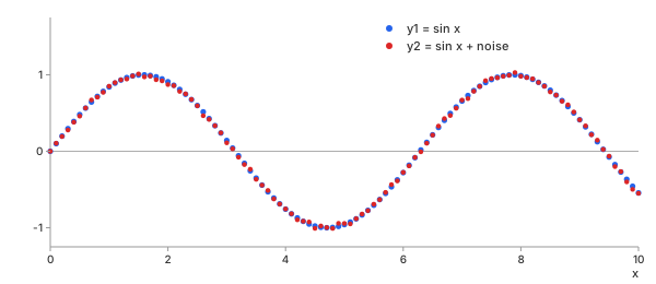
Chart 1. $y_1$ and $y_2$ of Table 1 at all 101 samples
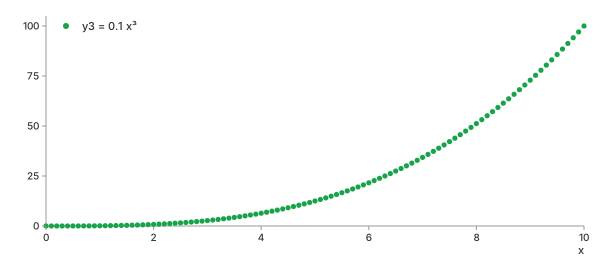
Chart 2. $y_3$ of Table 1 at all 101 samples
Chart 3 illustrates both operations using $y_1$ from Chart 1. At $x$ = 1, the blue line has the slope estimated by the numerical derivative: 0.539 (the true slope, $\cos 1$, is 0.540). The shaded region beneath the samples from $x$ = 2 to 3 represents the area estimated by numerical integration.
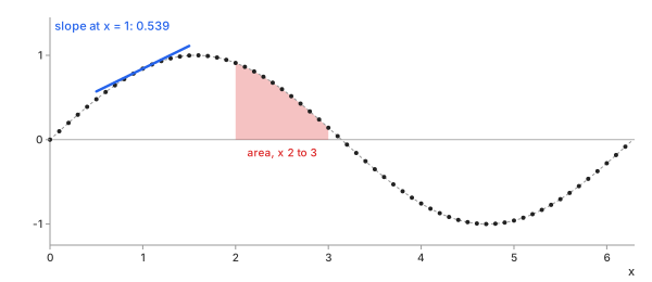
Chart 3. $y_1$ of Chart 1: the slope at one point, and the area over one range
All subsequent charts use the same $y_1$, $y_2$, and $y_3$ data.
Methods
The methods fall into two families. Derivatives subtract neighbouring samples and divide by the distance between them in $x$. Integrals add the areas of thin strips between neighbouring samples. Both operate directly on the data, without requiring an underlying formula.
Derivatives
Forward and Backward Difference
In plain words. The slope at a sample is the rise to the next sample divided by the run: the forward difference. Looking back to the previous sample instead gives the backward difference. Each uses one neighbour only, so each describes the slope at the midpoint of its chord, half a step away from the point it is reported at: there, at $x_i + h/2$ for the forward difference, it is second-order accurate; at $x_i$ itself only first-order.
Control parameters. method = forward or backward, and order ($n$, 1 by default; the advanced calculator only). There are no other settings: $h$ is determined by the spacing of the data.
Basic idea. With $h$ = $x_{i+1} - x_i$ (Math 1):
Math 1.
- Why a difference: The derivative is the limit of this ratio as the step approaches zero. With measured data, the step cannot be reduced beyond the available sample spacing, so the ratio is evaluated using that spacing.
- **Worked at $x$ = 1:** Table 2 uses the three samples of $y_1$ around $x$ = 1 from Table 1, with Math 1 and $h$ = 0.1. Compared with the true slope, the forward estimate is 0.043 too low and the backward estimate is 0.042 too high.
$$\begin{aligned} &\text{forward: } y'(1) \approx \frac{0.8912 - 0.8415}{0.1} = 0.4970 \\[0.9em] &\text{backward: } y'(1) \approx \frac{0.8415 - 0.7833}{0.1} = 0.5820 \\[0.9em] &\text{true: } \cos 1 = 0.5403 \end{aligned}$$$$\begin{aligned} &\text{forward:} \\ &y'(1) \approx \frac{0.8912 - 0.8415}{0.1} = 0.4970 \\[0.9em] &\text{backward:} \\ &y'(1) \approx \frac{0.8415 - 0.7833}{0.1} = 0.5820 \\[0.9em] &\text{true: } \cos 1 = 0.5403 \end{aligned}$$
- Picture: Chart 4 shows each estimated slope as a line through the sample at $x$ = 1. The forward line follows the chord to the right, while the backward line follows the chord to the left; the curve bends between the two neighbouring samples.
| method | samples of $y_1$ used | slope at $x$ = 1 | error against $\cos 1$ = 0.5403 |
|---|---|---|---|
| forward (Math 1) | $x$ = 1: 0.8415, $x$ = 1.1: 0.8912 | 0.4970 | −0.0433 |
| backward (Math 1) | $x$ = 0.9: 0.7833, $x$ = 1: 0.8415 | 0.5820 | +0.0417 |
| central (Math 2) | $x$ = 0.9: 0.7833, $x$ = 1.1: 0.8912 | 0.5395 | −0.0008 |
Table 2. Three samples of $y_1$ around $x$ = 1, and the slope each method takes from them
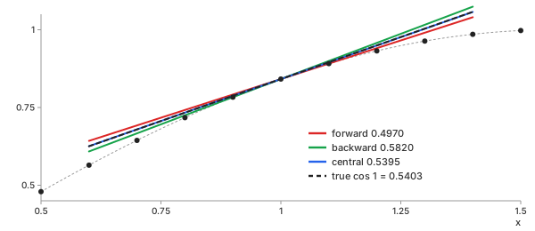
Chart 4. The slopes of Table 2 drawn through $y_1$ at $x$ = 1
Advantages
- Simple: one subtraction and one division per point.
- Causal: the backward difference uses only past samples, so it works on data arriving in real time. The forward and central differences need the next sample, which a live stream does not have yet: they are non-causal.
- Any spacing: each step uses its own $x_{i+1} - x_i$.
Disadvantages
- First order: the error decreases in proportion to $h$ (Order of Accuracy). Across the full $y_1$ record, the maximum error reaches 0.050 (Chart 5).
- Shifted: each result belongs half a step from the sample it is reported at.
- Noise: the largest of the four methods on noisy data (Table 4).
Central Difference
In plain words. Draw a chord between the sample before and the sample after, then use its slope at the central sample. The two one-sided errors of Table 2, one too low and one too high, cancel: the central difference is their average.
Control parameters. method = central, and
order ($n$). The basic calculator uses this method.
Basic idea. On evenly spaced data, with $h$ the constant step between neighbouring samples (Math 2; uneven spacing has its own form, Math 13):
Math 2.
- Why both sides: To first order, the curvature shifts the forward and backward estimates by equal amounts in opposite directions. Averaging the two therefore cancels this error.
- Worked at $x$ = 1: Math 2 on the same three samples (Table 2).
The error is fifty times smaller than either one-sided difference; in Chart 4 the blue
line is almost on the true tangent.
$$\begin{aligned} &y'(1) \approx \frac{0.8912 - 0.7833}{0.2} = 0.5395 \\[0.9em] &\text{error} = 0.5395 - 0.5403 = -0.0008 \end{aligned}$$
- Whole record: Chart 5 plots each method's error relative to $\cos x$ across all samples of $y_1$ in Chart 1. Forward and backward swing by ±0.050; central stays within 0.0020 inside the record.
- Edges: the first and last samples have only one neighbour, so there the central method falls back to the one-sided difference (Edges).
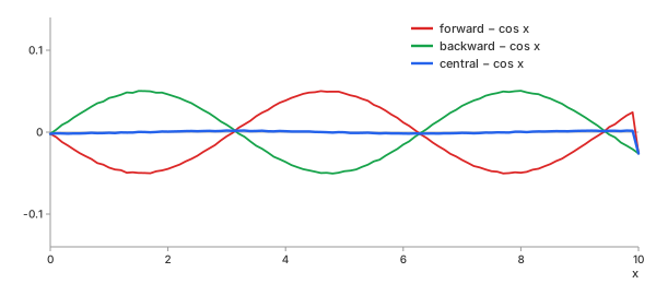
Chart 5. Error of forward, backward and central (Math 1, Math 2) on $y_1$, against the true $\cos x$
Advantages
- Second order: halve $h$ and the error falls by four.
- Centred: the result belongs to the sample it is reported at.
- Exact on a parabola: for any quadratic the curvature terms cancel completely.
Disadvantages
- Needs both neighbours: one-sided, and less accurate, at the two ends; and non-causal, since it waits for the next sample.
- Still noisy: on $y_2$ the error is 0.126 RMS, seven times the noise itself (Noise).
Second and Higher Derivatives
In plain words. The derivative of a derivative is the second derivative. It describes curvature, or acceleration when $y$ represents position. Numerically, it is obtained by applying the same differentiation step again to the first derivative.
Control parameters. order ($n$ below), 1 to 4, on the
advanced calculator. Order 2 runs the chosen method twice, order 4 four times.
Basic idea. Math 2 applied twice on even spacing reaches two samples to each side, with a step of $2h$ (Math 3, first line). The conventional three-point formula uses the nearest neighbours instead, with a step of $h$ (Math 3, second line). They are different formulas:
Math 3.
- Why apply it again: The same rule and edge treatment can be used at every order. For example, the calculator's third derivative applies the same differentiation step three times. The forward, backward, and central options are available at each order.
- Worked at $x$ = 1: the repeated form takes $y_1$ at 0.8, 1 and
1.2, the three-point form at 0.9, 1 and 1.1 (Table 1).
$$\begin{aligned} &\text{repeated: } y''(1) \approx \frac{0.9320 - 2(0.8415) + 0.7174}{4(0.01)} = -0.8400 \\[0.9em] &\text{three-point: } y''(1) \approx \frac{0.8912 - 2(0.8415) + 0.7833}{0.01} = -0.8500 \\[0.9em] &\text{true: } -\sin 1 = -0.8415 \end{aligned}$$$$\begin{aligned} &\text{repeated: } y''(1) \approx \\ &\frac{0.9320 - 2(0.8415) + 0.7174}{4(0.01)} \\ &= -0.8400 \\[0.9em] &\text{three-point: } y''(1) \approx \\ &\frac{0.8912 - 2(0.8415) + 0.7833}{0.01} \\ &= -0.8500 \\[0.9em] &\text{true: } -\sin 1 = -0.8415 \end{aligned}$$
- Which is more accurate: for exact $\sin x$, the three-point form is more accurate, with a truncation error four times smaller: 0.00058 RMS against 0.0023 inside the record. On $y_1$, stored to four decimals, the order flips: 0.0073 against 0.0029. Rounding contributes an effective noise level of 0.000029. The three-point formula divides this error by $h^2$ = 0.01, whereas the repeated formula divides it by $4h^2$ = 0.04.
- Picture: Chart 6 shows the result over all of $y_1$ in Chart 1, on the curve $-\sin x$; its error is 0.0029 RMS inside the record (rows 3 to 99, the two edge rows on each side left out).
- Each order costs: each pass introduces another division by $h$, so noise can grow rapidly with the derivative order (Higher Orders).
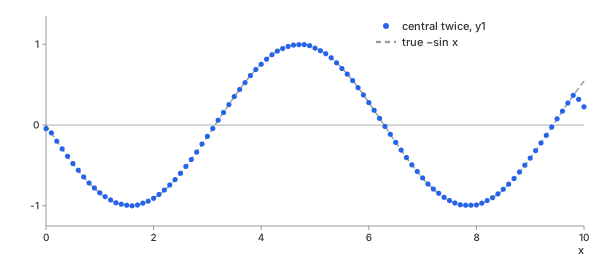
Chart 6. Central difference applied twice to $y_1$ (Math 3), against the true $-\sin x$
Advantages
- One rule: any order from one first-derivative method.
- Clean data: accurate to the same order as the method it repeats.
Disadvantages
- Wider reach: order $n$ reaches $n$ samples to each side, so the edge effect spreads $n$ samples in.
- Noise: roughly multiplied by $1/h$ per order; on $y_2$ the fourth derivative is 92 RMS off (Chart 17).
Savitzky-Golay Derivative
In plain words. Instead of drawing a chord through two samples, fit a polynomial to a window of samples using least squares, then calculate the polynomial's slope at the centre of the window. The fit reduces the effect of noise before the slope is calculated: a smoothed derivative, the derivative form of the Savitzky-Golay smoother.
Control parameters. window ($2k+1$ samples, odd, 9 by
default), polyorder ($p$, 3 by default; at least the order $n$), and
order ($n$). Advanced calculator only. It needs evenly spaced $x$.
Basic idea. Around sample $i$, with $t = (x - x_i)/h$, fit $\sum_{j=0}^{p} a_j t^j$ to the $2k+1$ samples $y_{i-k}, \dots, y_{i+k}$; the $n$-th derivative at the centre is read off one coefficient (Math 4):
Math 4.
- Why a fit: a chord through two noisy samples carries both samples' noise at full size. The polynomial is fitted by least squares to all nine samples, so the resulting slope is a fixed weighted sum of the nine samples. The weights are determined by
windowandpolyorder, and some may be negative. For window 9, polyorder 3, the weights times $h$ are 0.0724, −0.1195, −0.1625, −0.1061, 0, 0.1061, 0.1625, 0.1195, −0.0724. Noise of $\sigma$ on each sample comes out as 3.38$\sigma$, against the central difference's $\sigma/(\sqrt{2}h)$ = 7.07$\sigma$ at $h$ = 0.1. - **On $y_2$:** Chart 7 compares it with the central difference on the noisy $y_2$ of Chart 1. The central difference has an RMS error of 0.126 relative to $\cos x$. Savitzky-Golay with window 9 and polyorder 3 reduces it to 0.062, about half as large.
- Its order: one fit gives every derivative up to $p$ at once, so order $n$ is read off directly, not by repeating the method.
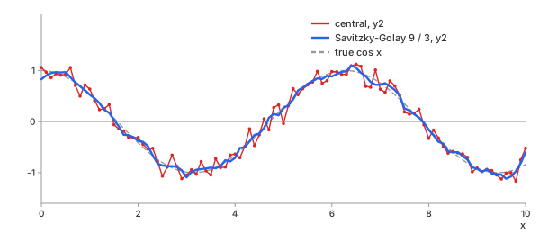
Chart 7. The derivative of $y_2$: central difference (Math 2) against Savitzky-Golay (Math 4), window 9, polyorder 3
Advantages
- Noise: the lowest error on noisy data of the four (Table 4).
- Clean data too: 0.0003 RMS on $y_1$, ten times better than central, since polyorder 3 follows the curvature.
Disadvantages
- Even spacing: the fit assumes one fixed $h$; the calculator refuses uneven $x$ for this method.
- Two knobs: a window too wide flattens sharp features; too narrow leaves the noise. See the smoothing article for how to pick them.
Integrals
Trapezoid Rule
In plain words. Connect neighbouring samples with straight lines. The area under each segment is a trapezoid: its width multiplied by the average of the two endpoint values. The total integral is the sum of these trapezoid areas.
Control parameters. method = trapezoid.
The range is set by from and to ($a$, $b$), the whole record
by default. The basic calculator uses this method.
Basic idea. (Math 5):
Math 5.
- Why straight lines: they are the simplest curve through two samples, and need no assumption about the spacing.
- Worked: Table 3 adds the first four panels of $y_1$ from Table 1, $x$ = 0 to 0.4. The resulting sum is 0.078870; the exact area, $1 - \cos 0.4$, is 0.078939.
- Picture: Chart 8 draws the ten panels from 0 to 1 under the samples of $y_1$. Each straight segment lies slightly below the sine curve, so the estimated area is a little too small.
| panel | $x_i$ to $x_{i+1}$ | $y_i$, $y_{i+1}$ | area |
|---|---|---|---|
| 1 | 0 to 0.1 | 0.0000, 0.0998 | 0.004990 |
| 2 | 0.1 to 0.2 | 0.0998, 0.1987 | 0.014925 |
| 3 | 0.2 to 0.3 | 0.1987, 0.2955 | 0.024710 |
| 4 | 0.3 to 0.4 | 0.2955, 0.3894 | 0.034245 |
| sum | 0 to 0.4 | 0.078870 |
Table 3. Math 5 on the first four panels of $y_1$
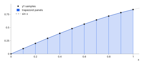
Chart 8. The trapezoid panels (Math 5) under $y_1$ from $x$ = 0 to 1
Advantages
- Any spacing: each panel has its own width.
- Robust: never overshoots between samples.
- Exact on straight lines.
Disadvantages
- Second order: on curved data it misses the bend; on $y_3$ it is 0.025 too high out of 250 (Table 5).
Simpson's Rule
In plain words. Replace the straight segments with parabolas, each passing through three neighbouring samples. A parabola follows the curve's bend more closely, generally giving a more accurate area estimate.
Control parameters. method = simpson, on
the advanced calculator, with from and to as for the
trapezoid.
Basic idea. On even spacing, with $h$ the constant distance between neighbouring samples ($h = x_{i+1} - x_i$ = $x_i - x_{i-1}$, the width of one panel), each pair of panels, from $x_{i-1}$ to $x_{i+1}$, contributes (Math 6):
Math 6.
- Why a parabola: Three samples determine a unique parabola. Integrating it gives this formula, with weights 1, 4, and 1.
- Picture: Chart 9 takes $\sin x$ at only five points, $x$ = 0 to 4 with $h$ = 1, to make the difference visible: the straight lines cut under the arch, the two parabolas follow it.
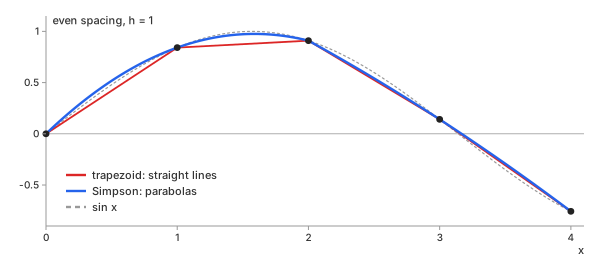
Chart 9. $\sin x$ at $h$ = 1: trapezoid lines (Math 5) against Simpson's parabolas (Math 6)
- Worked on Chart 9: Math 6 on its two pairs of panels, 0 to 2 and 2 to 4; the middle sample at $x$ = 2 is shared by both pairs and contributes to each pair's estimate.
$$\begin{aligned} &\text{pair } 0 \text{ to } 2: \ \tfrac{1}{3}\big(0 + 4(0.8415) + 0.9093\big) = 1.4251 \\[0.9em] &\text{pair } 2 \text{ to } 4: \ \tfrac{1}{3}\big(0.9093 + 4(0.1411) - 0.7568\big) = 0.2390 \\[0.9em] &\text{sum: } 1.4251 + 0.2390 = 1.6641 \\[0.9em] &\text{trapezoid: } 1.5135 \\[0.9em] &\text{true: } 1 - \cos 4 = 1.6536 \end{aligned}$$$$\begin{aligned} &\text{pair } 0 \text{ to } 2: \\ &\tfrac{1}{3}\big(0 + 4(0.8415) + 0.9093\big) \\ &= 1.4251 \\[0.9em] &\text{pair } 2 \text{ to } 4: \\ &\tfrac{1}{3}\big(0.9093 + 4(0.1411) - 0.7568\big) \\ &= 0.2390 \\[0.9em] &\text{sum: } 1.4251 + 0.2390 = 1.6641 \\[0.9em] &\text{trapezoid: } 1.5135 \\[0.9em] &\text{true: } 1 - \cos 4 = 1.6536 \end{aligned}$$
- Exact on cubics, on even spacing: with an even number of panels, Math 6 is exact for any cubic. On $y_3$ of Chart 2, 100 panels, it gives 250.000000, the exact area (Table 5).
- Odd number of panels: Math 6 needs panels in pairs. The calculator uses SciPy's Simpson, which then integrates the last panel with Cartwright's correction instead. On $y_3$ from 0 to 9.9, 99 panels: 240.149005 against the exact 240.149003.
Uneven spacing. When the two panels in a pair have different widths, with $h_- = x_i - x_{i-1}$ and $h_+ = x_{i+1} - x_i$, the parabola through the three samples gives Math 7; with $h_- = h_+ = h$ it turns back into Math 6:
Math 7.
- Worked on uneven $x$: Chart 10 takes $\sin x$ at $x$ = 0, 0.6 and
2.0: 0, 0.5646 and 0.9093, so $h_-$ = 0.6 and $h_+$ = 1.4. Math 7 piece by piece: the
factor in front, the three brackets, the three weights (factor times bracket), then
the sum. The first weight is negative: when one panel is much wider than the other, a
sample's weight can drop below zero.
$$\begin{aligned} &\frac{h_- + h_+}{6} = \frac{0.6 + 1.4}{6} = 0.3333 \\[0.9em] &2 - \frac{h_+}{h_-} = 2 - \frac{1.4}{0.6} = -0.3333 \\[0.9em] &\frac{(h_- + h_+)^2}{h_- h_+} = \frac{2.0^2}{0.6 \times 1.4} = 4.7619 \\[0.9em] &2 - \frac{h_-}{h_+} = 2 - \frac{0.6}{1.4} = 1.5714 \\[0.9em] &\text{weights: } {-0.1111},\ 1.5873,\ 0.5238 \\[0.9em] &\text{area} \approx -0.1111(0) + 1.5873(0.5646) + 0.5238(0.9093) = 1.3725 \\[0.9em] &\text{trapezoid: } 1.2011 \\[0.9em] &\text{true: } 1 - \cos 2 = 1.4161 \end{aligned}$$$$\begin{aligned} &\frac{h_- + h_+}{6} = \frac{0.6 + 1.4}{6} = 0.3333 \\[0.9em] &2 - \frac{h_+}{h_-} = 2 - \frac{1.4}{0.6} = -0.3333 \\[0.9em] &\frac{(h_- + h_+)^2}{h_- h_+} = \frac{2.0^2}{0.6 \times 1.4} = 4.7619 \\[0.9em] &2 - \frac{h_-}{h_+} = 2 - \frac{0.6}{1.4} = 1.5714 \\[0.9em] &\text{weights: } {-0.1111},\ 1.5873,\ 0.5238 \\[0.9em] &\text{area} \approx -0.1111(0) \\ &\qquad + 1.5873(0.5646) \\ &\qquad + 0.5238(0.9093) \\ &\qquad = 1.3725 \\[0.9em] &\text{trapezoid: } 1.2011 \\[0.9em] &\text{true: } 1 - \cos 2 = 1.4161 \end{aligned}$$
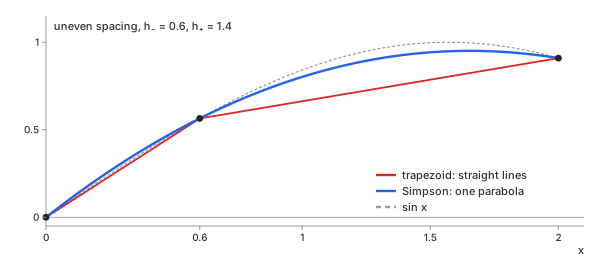
Chart 10. One uneven pair of panels, $h_-$ = 0.6 and $h_+$ = 1.4: trapezoid lines (Math 5) against Simpson's parabola (Math 7)
- **Uneven $x$, exactness:** each parabola is fitted using the actual positions of its three samples. The resulting rule is exact for quadratic functions, but not generally for cubics. On 41 random $x$ from 0 to 10: a quadratic integrates to 100.000000 (exact 100), the cubic $0.1x^3$ to 249.980536 (exact 250).
Advantages
- Fourth order on evenly spaced data: halving $h$ reduces the error by a factor of sixteen, under the usual smoothness conditions.
- Exact for cubics: with evenly spaced samples and an even number of panels.
Disadvantages
- Can overshoot: a parabola through a sharp corner or a noise spike bulges past the data.
- No noise reduction: its advantage is better representation of curvature, not noise reduction. Its weights, $h/3$ times 1, 4, 2, 4, …, 1, even pass slightly more of the samples' noise than the trapezoid's $h/2$ times 1, 2, 2, …, 1: on noise alone, $\sigma$ = 0.02 on every sample, the total from 0 to 10 scatters by 0.0206, against the trapezoid's 0.0195, about 5 % more.
Cumulative Integral
In plain words. Rather than calculating only one total, maintain a running sum and report it at every sample. The result is a new curve whose value at each $x$ is the accumulated area from the first sample to that point. This is the curve shown in the calculators' output grid.
Control parameters. method (trapezoid or Simpson),
order ($n$), and constants ($C$, 0 by default; advanced
calculator).
Basic idea. Start at $C$ and add one panel at a time (Math 8):
Math 8.
- Why a curve: the integral of position-dependent data is itself position-dependent: the energy used so far, the distance travelled so far.
- On $y_1$: Chart 11 shows the cumulative trapezoid of $y_1$ from Chart 1, on the true $1 - \cos x$. The running sums of Table 3 are its first five values; the last value, 1.8375, is the total over the whole record (true 1.8391).
- The constant: $C$ shifts the whole curve up or down (Integration Constant and Area).
- Cumulative Simpson: on the advanced calculator, each panel's
strip is the area under a parabola through three neighbouring samples, the third chosen
alternately: panels 1, 3, 5, … take the panel's two samples and the next one; panels
2, 4, 6, … the previous one and the panel's two; the last panel, having no next sample,
always takes the previous one (SciPy's
cumulative_simpson, after Cartwright). Each strip is then exact only for quadratics: on $y_3$ the running values miss $0.025x^4$ by up to 0.0000025, while the value at $x$ = 10, the whole-record total, is still exactly 250.
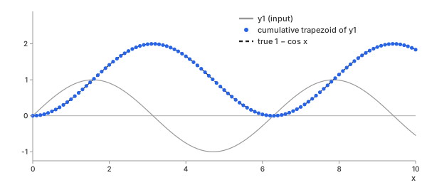
Chart 11. The cumulative trapezoid integral (Math 8) of $y_1$, against the true $1 - \cos x$
Advantages
- Every range at once: the area between any two sample positions is the difference between the corresponding values of the cumulative integral.
- Smooth: summing averages the noise (Chart 16).
Disadvantages
- Drift: any constant offset in $y$, a detector bias for example, adds a straight line that grows with $x$.
- Starts at a choice: the curve's level depends on $C$, which the data cannot tell.
Which One Should You Choose?
For derivatives, Table 4 lists each method's RMS error relative to $\cos x$ for $y_1$ and $y_2$ from Chart 1. Chart 12 presents the same results graphically.
| method | $y_1$, clean | $y_2$, noisy | use when |
|---|---|---|---|
| forward (Math 1) | 0.0344 | 0.2480 | data arriving in time, only the past known |
| backward (Math 1) | 0.0344 | 0.2454 | same |
| central (Math 2) | 0.0029 | 0.1259 | the default: any spacing, clean data |
| Savitzky-Golay (Math 4) | 0.0003 | 0.0621 | noisy data, even spacing |
Table 4. Derivative methods: RMS error against $\cos x$ over all 101 samples, edges included
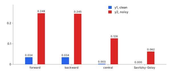
Chart 12. Table 4 as bars
For integrals, Table 5 lists the error in the total over the full record for $y_1$ (exact value $1 - \cos 10$ = 1.839072) and $y_3$ (exact value 250). Chart 13 presents these results graphically.
| method | $y_1$ | $y_3$ | use when |
|---|---|---|---|
| trapezoid (Math 5) | 0.0016 | 0.025 | the default: any data, never overshoots |
| Simpson (Math 6) | 0.000045 | 0 | smooth, curved data |
Table 5. Integral methods: error of the total
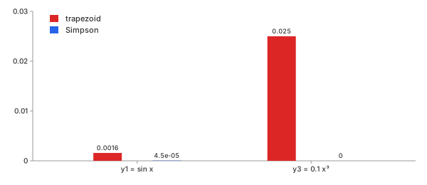
Chart 13. Table 5 as bars
Start with the central difference for derivatives and the trapezoid rule for integrals; both handle uneven spacing. Use Savitzky-Golay when the derivative is noisy, and Simpson's rule when the data is smooth and greater accuracy in the total area is important.
Key Ideas
Step Size: The Smallest Is Not the Best
When working with a formula, you can choose the step $h$. A smaller step generally reduces the truncation error—the error caused by approximating the curve with a chord. With measured data, however, each sample also contains noise, represented here by $\varepsilon$, the typical error in an individual sample. Differentiation divides the difference between samples by $h$, amplifying this noise. The total error of the central difference has both parts (Math 9), where $|y'''|$ is the size of the third derivative near the point. Math 9 is an approximation. It assumes that $y'''$ varies little over the chord and that the noise has roughly the same magnitude at each sample.
Math 9.
Chart 14 illustrates this behaviour using $\sin x$ sampled at 200 points, with step sizes ranging from 0.0001 to 1. Without noise (blue) the error falls with $h^2$ down to $9.4 \times 10^{-10}$. With noise of 0.001 (red) it falls only until $h$ ≈ 0.18, then rises again: at $h$ = 0.0001 it is 5.6, larger than the slope itself. Math 9 predicts $h^{*}$ ≈ 0.14 for $\varepsilon$ = 0.001 and $|y'''| \le 1$: the same size.
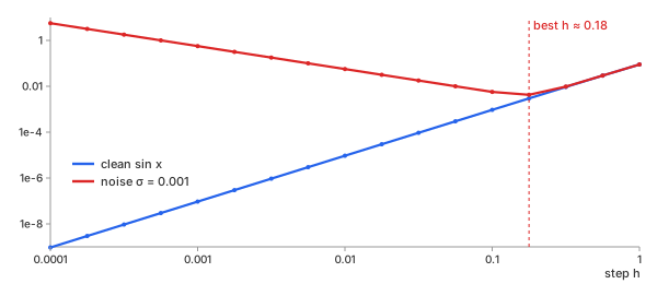
Chart 14. Central difference (Math 2) on $\sin x$: error against step $h$, clean and with noise 0.001 (Math 9)
Chart 14 chooses the step freely, as one can with a formula. With data, the sampling interval (0.1 in the example) fixes the smallest differentiation step: the central difference's chord spans two intervals. A wider step is still possible, by taking the chord to samples $k$ rows away, which trades truncation error for less noise exactly as Chart 14 shows. The other knob is to reduce $\varepsilon$ first: smooth, or use Savitzky-Golay.
Order of Accuracy
The order of a method is the power $p$ that describes how its error decreases as the step size is reduced (Math 10). Halving $h$ reduces the error by a factor of $2^p$.
Math 10.
Chart 15 measures $p$ on clean $\sin x$ over 0 to $\pi$: the derivative at $x$ = 1, the integral over the whole range (true value 2). On log-log axes each error is a straight line whose slope is $p$: forward 1.01, central 2.00, trapezoid 2.00, Simpson 4.00. At $h$ = 0.0245 Simpson's error is $4.0 \times 10^{-9}$, the trapezoid's $1.0 \times 10^{-4}$.
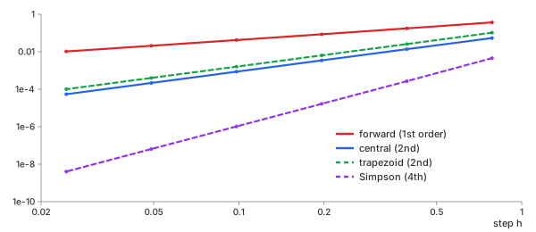
Chart 15. Error against step $h$ on clean $\sin x$: the slope of each line is the order $p$ (Math 10)
This order-of-accuracy description applies to clean, smooth data. With noisy data, the noise term in Math 9 can dominate, so using a higher-order method does not necessarily improve the result.
Noise: Derivatives Amplify, Integrals Average
A derivative subtracts two nearby values. Much of the underlying signal cancels, but the noise generally does not; the remaining difference is then divided by a small step size. With independent, zero-mean noise of standard deviation $\sigma$ on each sample, the central difference carries (Math 11):
Math 11.
An integral scales each sample's noise by approximately $h$ and accumulates the contributions. For independent, zero-mean errors, positive and negative contributions partly cancel, so the resulting standard deviation grows approximately with the square root of the number of panels, $N$. Chart 16 shows both on $y_2$ of Chart 1, whose noise is 0.0178 RMS: the derivative has an RMS error of 0.126, about seven times the noise level, as predicted by Math 11. The integral's RMS error is 0.027 and varies much more gradually.
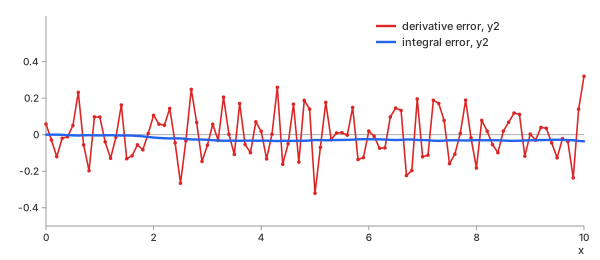
Chart 16. $y_2$: error of the central derivative and of the cumulative trapezoid integral (Math 11)
- Frequency view: differentiating a sinusoidal component with angular frequency $\omega$ multiplies its amplitude by $\omega$; the central-difference operator instead has a frequency response proportional to $\sin(\omega h)/h$, which approaches $\omega$ at low frequencies. For a nonzero-frequency component, integration scales its amplitude by $\omega$. White noise contains components across the sampled frequency range, and differentiation weights higher frequencies more strongly while integration attenuates them. This helps explain the jagged red derivative and smoother blue integral in Chart 16.
- Correlated noise: Math 11 assumes that the error at each sample is independent. If neighbouring errors move together, the noise varies more slowly: differentiation is less affected because the difference cancels the shared component, while integration is more affected. Its error can then grow in proportion to $N$, rather than $\sqrt{N}$.
- Systematic offset: a constant bias $c$ in $y$ does not affect the derivative, but it adds $c\,(x - x_0)$ to the integral, producing a linear drift across the record. A linear drift in $y$ adds a constant to the derivative. Remove the baseline before integrating when it is not part of the signal.
Higher Orders
The advanced calculator can repeat each operation up to four times. The $n$-th derivative applies the first-derivative operation $n$ times. The $n$-th integral applies cumulative integration $n$ times, with the $k$-th pass starting from its own constant $C_k$ (Math 12):
Math 12.
The independent-noise estimate in Math 11 does not apply unchanged at every pass: each operation changes the correlations between errors in neighbouring samples. Chart 17 reports the measured RMS error for $y_2$ from Chart 1, for orders $n$ = 1 to 4, relative to the exact derivatives of $\sin x$ and its repeated integrals (with all $C_k$ = 0). The derivative error grows by roughly a factor of nine at each order: 0.13, 1.1, 9.8, and 92. The integral error also grows, but remains small relative to the values themselves: 0.027, 0.13, 0.40, and 0.93, compared with a fourth integral that reaches 156 at $x$ = 10.
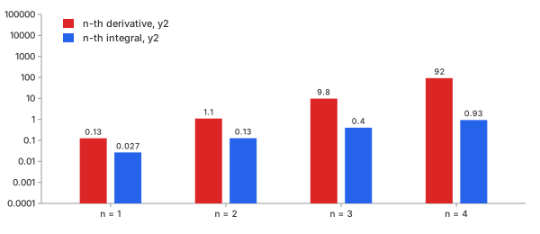
Chart 17. $y_2$: RMS error of the $n$-th derivative and the $n$-th integral (Math 12)
For measured data, even a second derivative can be unreliable without smoothing; a fourth derivative may be dominated by noise. Repeated integrals stay usable. The units follow the order: the $n$-th derivative is in $y$ per $x^n$, the $n$-th integral in $y$ times $x^n$. With $y$ a position in metres and $x$ a time in seconds, the derivative is a velocity in m/s and the second derivative an acceleration in m/s², while the integral is in m·s. With $y$ a power in watts and $x$ in hours, the integral is an energy in watt-hours (W·h), while the derivative is a rate of change of power in W/h.
Uneven x
Measured data is not always evenly spaced: a data logger may skip samples, or a measurement sweep may slow down. The trapezoid rule (Math 5) uses the actual width of each panel and requires no further assumptions about spacing. For unevenly spaced data, the central-difference formula accounts for the different distances to the two neighbouring samples ($h_-$ = $x_i - x_{i-1}$, $h_+$ = $x_{i+1} - x_i$), and is still second order (Math 13):
Math 13.
With $h_-$ = $h_+$ it is Math 2 again. Its truncation error is about $(h_- h_+/6)\,|y'''|$, so it stays second order in the larger step as the sampling is refined, as long as neighbouring steps stay comparable. A very uneven pair still converges, but its weights grow like $1/\min(h_-, h_+)$: noise on the sample beside the short step is amplified most. Every method needs $x$ strictly increasing: the calculators sort the rows by $x$ and refuse a repeated $x$, whose step of zero would divide by zero. Chart 18 samples $\sin x$ at 25 random points, with steps from 0.01 to 1.18: the central difference still lands on $\cos x$, 0.023 RMS inside the record. Savitzky-Golay and Simpson's even-spacing form (Math 4, Math 6) assume one step; the calculator refuses uneven $x$ for Savitzky-Golay and uses SciPy's uneven-spacing Simpson.
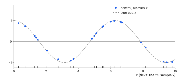
Chart 18. $\sin x$ at 25 uneven points: central difference (Math 13) against $\cos x$
Edges
The first sample has no neighbour to its left, and the last has none to its right. The calculators do not invent missing samples. At either endpoint, every difference method uses the one-sided difference from Math 1, directed into the data range. This estimate is first-order accurate: its error is approximately $(h/2)\,|y''|$, compared with $(h^2/6)\,|y'''|$ for the central difference at interior points. In Chart 5, this appears as the jump at $x$ = 10. The error at the last sample is −0.0259, close to the estimate below and about thirteen times the 0.0020 RMS error of the central difference in the interior. (At $x$ = 0 the one-sided error happens to be small, −0.0020, because $\sin x$ has no curvature there.) Each additional differentiation pass extends the affected edge region by one sample: in Chart 6 the second derivative is off by 0.045 at $x$ = 0. Read the values near both ends with care, and more of them the higher the order.
Integration Constant and Area
The cumulative integral (Math 8) starts from a constant $C$, which cannot be determined from the measured data alone. It may represent, for example, the initial position or the charge already stored. Chart 19 shows the cumulative integral of $y_1$ from Chart 1 for $C$ = 0 and $C$ = −1. The two curves have the same shape and differ only by a vertical shift. Between $x$ = 2 and 6 both change by exactly the same amount, −1.3752: from 1.4150 to 0.0398, and from 0.4150 to −0.9602.
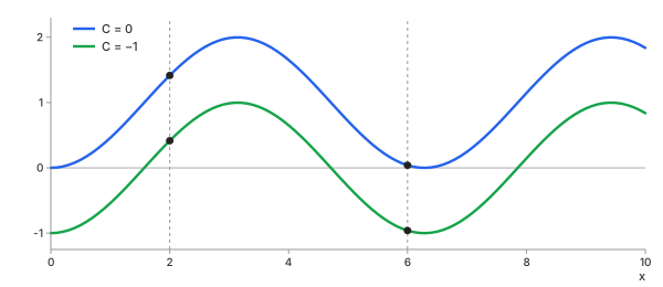
Chart 19. The cumulative integral (Math 8) of $y_1$ with two constants: the change from $x$ = 2 to 6 is the same
This change is the area over the selected range; the integration constant cancels out. The calculators report it under the chart for any range you set. The calculators report two forms of area (Math 14): signed area, where regions below the axis subtract from those above it, and absolute area, where all regions contribute positively:
Math 14.
Chart 20 shades $y_1$ from 2 to 6: blue above the axis, red below. Signed, the red outweighs the blue: −1.3752 (true $\cos 2 - \cos 6$ = −1.3763). Absolute, both add: 2.5419 (true 2.5440). Net charge is signed; total distance travelled, whatever the direction, is absolute. For the absolute area the calculators split each panel where it crosses zero, so no panel cancels itself. A range end between two samples takes the straight line between them. On the advanced calculator at order $n$ > 1, the area is taken under the $(n-1)$-th integral, so that it equals the change of the $n$-th one.
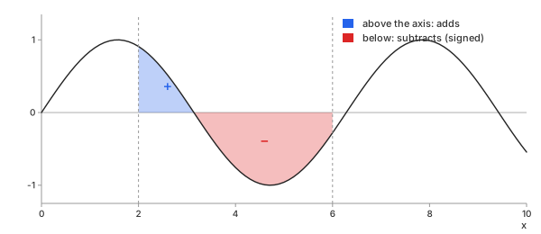
Chart 20. $y_1$ from $x$ = 2 to 6: area above the axis adds, below subtracts in the signed area (Math 14)
Example: One Noisy Record, Differentiated and Integrated
Consider again $y_2$ from Chart 1, the noisy sine wave. Table 6 lists the central-difference derivative and cumulative trapezoid integral at each integer value of $x$, alongside their exact values. Chart 21 shows all 101 samples for both results.
| $x$ | $y_2$ | derivative | $\cos x$ | integral | $1 - \cos x$ |
|---|---|---|---|---|---|
| 0 | 0.0000 | 1.0580 | 1.0000 | 0.0000 | 0.0000 |
| 1 | 0.8513 | 0.6370 | 0.5403 | 0.4557 | 0.4597 |
| 2 | 0.8725 | −0.3100 | −0.4161 | 1.4004 | 1.4161 |
| 3 | 0.1105 | −1.0475 | −0.9900 | 1.9619 | 1.9900 |
| 4 | −0.7546 | −0.6350 | −0.6536 | 1.6207 | 1.6536 |
| 5 | −0.9437 | −0.0370 | 0.2837 | 0.6872 | 0.7163 |
| 6 | −0.2754 | 0.9800 | 0.9602 | 0.0149 | 0.0398 |
| 7 | 0.6699 | 0.6330 | 0.7539 | 0.2171 | 0.2461 |
| 8 | 0.9808 | −0.3280 | −0.1455 | 1.1159 | 1.1455 |
| 9 | 0.4116 | −0.9080 | −0.9111 | 1.8804 | 1.9111 |
| 10 | −0.5501 | −0.5190 | −0.8391 | 1.8027 | 1.8391 |
| RMS error | 0.1259 | 0.0267 | |||
Table 6. $y_2$: central derivative (Math 2) and cumulative trapezoid integral (Math 8) against the truth
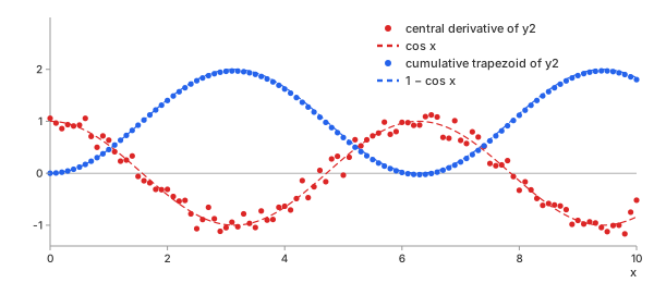
Chart 21. $y_2$: its derivative and integral (dots) against the true curves (dashed)
At $x$ = 5, the estimated derivative even has the wrong sign: −0.037, compared with the true slope of +0.284. The integral at the same point is off by 0.029. The same noise level (RMS 0.0178) produces an RMS error of 0.126 in the derivative and 0.027 in the integral (Math 11). For $y_2$, Savitzky-Golay reduces the derivative error by about half (Table 4). To obtain an even cleaner derivative, smooth the data first, or fit a model and differentiate the model instead: smoother, but only as right as the model.
Differentiate with care, integrate with confidence. The derivative of measured data can be dominated by noise unless that noise is reduced first.
REFs
Wikipedia, Finite difference Wikipedia, Numerical differentiation Wikipedia, Trapezoidal rule Wikipedia, Simpson's rule Wikipedia, Savitzky–Golay filter NIST DLMF §3.4, Differentiation NIST DLMF §3.5, Quadrature NumPy numpy.gradient SciPy scipy.integrate.trapezoid SciPy scipy.integrate.simpson SciPy scipy.integrate.cumulative_trapezoid SciPy scipy.integrate.cumulative_simpson SciPy scipy.signal.savgol_filter Smoothing Interpolation Curve Fitting: Which Equation Fits My Data, and How Well?